What are CpG islands and how to track them using a Hidden Markov Model?
It is sometimes relevant to predict the presence of genomic DNA features such as promoters, enhancers, silencers, insulators
and locus control regions. Such regulatory elements are called cis-regulatory modules or cis-regulatory switches. Identifying
them is difficult compared to finding protein-coding genes because the DNA sequences of interest may be very short (e.g. a
dozen base pairs for transcription factor-binding sites).
The dinucleotide CG is often referred to as CpG (p denotes the phosphate linkage between two desoxyriboses residues).
CpG islands represent an example of a regulatory element that are found in around \(70\%\) of the genes of eukariotic chromosomes.
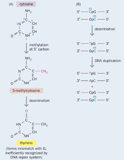
The dinucleotide cytosine followed by guanosine (CpG) is approximately five-fold underrepresented in many genomes, partly
because the cytosine residue can be exchanged for thymidine by spontaneous deamination, as shown in the figure on the right (credits:
Strachan, T. and Read, A. Human Molecular Genetics. 4ed. (2011), Box 9.1. Figure 1, p.262). CpG dinucleotides
are gradually being replaced by TpG and CpA. That is the reason why they are underepresented, unless other selection forces
act upon preserving the CpG dinucleotides.
Cytosine residues on CpG dinucleotides
are often methylated. This in turn leads to the recruitment of protein complexes that include histone diacetylases capable of
removing acetyl groups of histones and therefore inhibiting active transcription. Why is that? Acetylated histones carry negative
charges on the \(-CH_3-COO^-\) groups repelling the negative charges of the external phosphates groups in the double stranded DNA.
So when the acetyl groups are removed from histones associated to particular methylated regions in dsDNA, these regions tend to
better bind to histones, preventing access of transcription factors on these regions of the DNA. Hence, unmethylated CpG
dinucleotides do not recruit histone diacetylases and so enable easier access of transcription factors to the dsDNA without
having to deal with histones high intensity binding to the DNA sequence to be transcribed.
CpG islands are regions of high density of
unmetylated CpG dinucleotides and are commonly found in upstream (5') regulatory regions near the transcription start sites of
constitutively active 'housekeeping' genes.
By one criterion, a CpG island is defined as having:
- a GC content \(\ge 50\%\)
- a length \(\ge 200\, bp\)
- a ratio of observed to expected number of CpG dinucleotides of \(>0.6\).
As an example here, we will focus on the GDF15 gene (Growth Differentiation Factor 15). The UCSC Genome browser shows this
gene is on the forward strand of chromosome 19,
band p13.11. In the human genome reference GRch38/hg38, the physical position is located between 18.385 Mb and 18.450 Mb.
The UCSC browser shows there are 2 exons and 1 intron for the GDF15 gene (exon 1 is 309 nt starting at bp 18,386,158 and exon 2 is 891 nt
starting at bp 18,388,286). By checking 'show' in the CpG islands option in the 'regulation' section
of the UCSC Genome browser, two CpG island sequences are indicated in the gene. We will try to retrieve these CpG islands after
importing the DNA sequence locally on a laptop in FASTA format and screening with a self-made HMM algorithm in Python.
This GDF15 gene encodes a secreted ligand of the TGF\(\beta\) (Transforming Growth Factor-\(\beta\)) superfamily of proteins.
Ligands of this family bind various TGF\(\beta\) receptors leading to recruitment and activation of SMAD family transcription
factors that regulate gene expression.
The encoded preproprotein is proteolytically processed to generate each subunit of the disulfide-linked homodimer.
The protein is expressed in a broad range of cell types, acts as a pleiotropic cytokine and is involved in the stress response
program of cells after cellular injury. Increased protein levels are associated with disease states such as tissue hypoxia,
inflammation, acute injury and oxidative stress.
The size and locus positions identified by the UCSC genome browser for the two CpG islands are: CpG island of size 206 bp and
CpG island of size 600 bp at physical positions: chr19: 18,386,254-18,386,479 and chr19: 18,388,288-18,388,887 respectively.
These 2 CpG islands are thus located inside exon 1 and exon 2 of GDF15 respectively.
What is a Hidden Markov Model?
To design a Hidden Markov Model (HMM) algorithm to detect CpG islands in a genomic sequence, we first recall, in an
intuitively simple way, what a HMM is, as nicely explained in the book by Jones and Pevzer, taking the
fair bet casino example.
Credits: Jones, N.C and Pevzner, P.A. An introduction to Bioinformatics Algorithms.
Chap. 11: Hidden Markov Models. MIT Press, 2004.
An HMM can be viewed as an abstract machine that has the ability to produce some output using special coin tossing.
The operation of the machine proceeds in discrete steps: at the beginning of each step, the machine is in a
hidden state. There are \(k\) such hidden states. During the step, the HMM makes two decisions:
- (1) What state shall I move next?
- (2) What symbol - from an alphabet \(\Sigma\) - shall I emit?
In our CpG island example, there are 2 hidden states (are you in or are you out of a CpG island?) and the alphabet
is the set of all possible pairs of nucleotides (there are 16 such pairs: AA, CC, GG, TT, AC, AG, AT, CA,
CG, CT,
GA, GC, GT, TA, TC, TG). Depending on whether or not the hidden state is a CpG island, the probability to emit
the particular dinucleotide
CG will not be the same as compared to the other dinucleotides elements of the set.
The HMM decides on question (1) by choosing randomly among the \(k\) states (possibly by following a multinomial
distribution: each of the \(k\) states are not necessarily chosen with the same probability, or by following a
uniform distribution if all hidden states were equiprobable); then it decides on question (2) by choosing randomly among the
\(\Sigma\) symbols. The choice that the HMM makes are typically biased (the uniform distribution is not mandatory).
One key feature of a HMM is that the probability distributions that govern which state to move to
and which symbols to emit change from state to state. In essence, if there are \(k\) states, then there
are \(k\) different 'next state' distributions and \(k\) different 'symbol emission' distributions. Another
important feature of HMM is that an external observer can only see the emitted symbols but has no ability to see
what state the HMM is in at any step, hence the name Hidden Markov Model. The goal of the observer is
to infer the most likely states of the HMM by analysing the sequences of emitted symbols.
Since an HMM effectively uses dice to emit symbols, the sequence of symbols it produces does not form any
readily recognizable pattern.
Formally, an HMM \(\textit(M)\) is defined by an alphabet of emitted symbols \(\Sigma\),
a set of hidden states \(\textit(Q)\), a squared matrix of state transition probabilities \(\textit(A)\),
and a non necessarily squared matrix of emission probabilities \(\textit(E)\), where
- \((\Sigma)\) is an alphabet of symbols;
- \(\textit(Q)\) is a set of (hidden) states, each of which will emit symbols from the alphabet \(\Sigma\);
- \(\textit(A) = (a_{kl})\) is a \(Q\) by \(Q\) matrix describing the probability of
changing to state \(l\) after the HMM is in state \(k\); and
- \(\textit(E) = (e_k(b))\) is a \(Q\) by \(\Sigma\) matrix describing the probability of emitting
the symbol \(b\) during a step in which the HMM is in state \(k\).
Each row of the matrix \(\textit(A)\) describes a 'state die' (= singular of 'dice') with \(Q\)
sides, while each row of the matrix \(E\) describes a 'symbol die' with \(\Sigma\) sides.
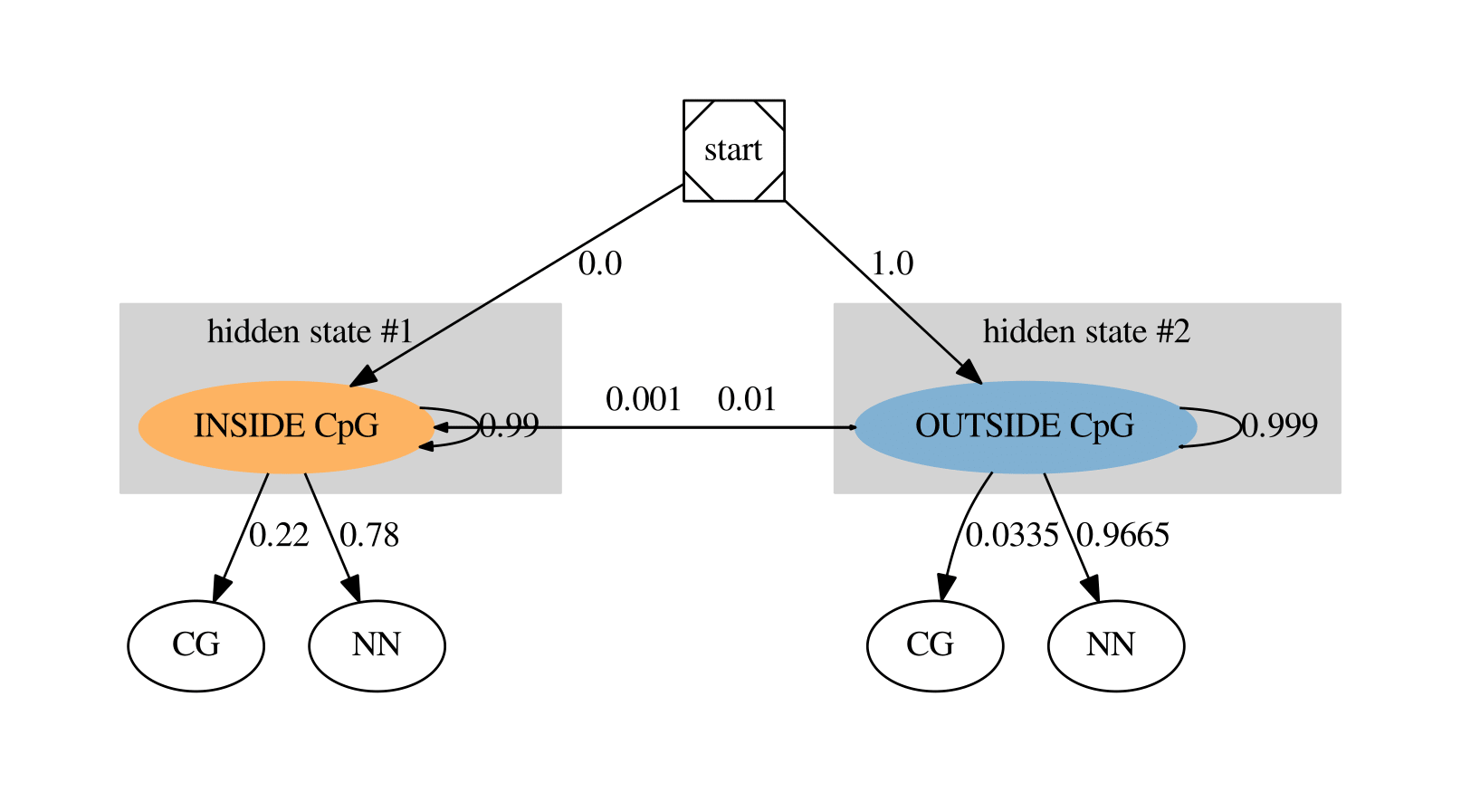
In our CpG island problem, the alphabet symbols are all possible dinucleotides \(\Sigma\)= AA, CC, GG, TT, AC, AG, AT, CA,
CG, CT,
GA, GC, GT, TA, TC, TG. For the sake of simplicity, we collapsed all non CG dinucleotides in the symbol 'NN', so
\(\Sigma = \) [CG, NN].
\(\textit Q\), the set of (hidden) states has the two states: inside (\(k=1\)) or outside a CpG island (\(k=0\)).
The 2 by 2 state transition matrix has 4 elements with the probabilities of the transitions between states (first row: \(k=0\);
second row: \(k=1\)) and writes:
\(A = a_{kl} =
\left(
\begin{array}{cc}
a_{00} & a_{01} \\
a_{10} & a_{11}
\end{array}
\right)
=
\left(
\begin{array}{cc}
0.999 & 0.001 \\
0.01 & 0.99
\end{array}
\right)\)
where, for instance, \(a_{10}=0.01\) is the probability to move from inside a CpG island to outside.
This was computed knowing that the mean 'duration' in state \(k\) is \(\bar d_k = \frac{1}{1\,-\,a_{kk}}\).
Considering that we require the minimum length of a CpG island to be 200 nucleotides, the number of steps
where the state should remain in a CpG island is around 100 (\(100 \times\, 2\) nucleotides), and so the
probability \(a_{11} = 0.99\). The probability to stay outside a CpG island is larger though.
The 2 by 2 matrix \(E\,=\,e_k(b)\), describing the probability of emitting a dinucleotide symbol
b
during a step in which the HMM is in state \(k\) writes:
\(E = e_k(b) =
\left(
\begin{array}{cc}
e_{0}(NN) & e_{0}(CG) \\
e_{1}(NN) & e_{1}(CG)
\end{array}
\right)
=
\left(
\begin{array}{cc}
0.9665 & 0.0335 \\
0.78 & 0.22
\end{array}
\right)
\)
The HMM has to start somewhere and we hypothesized that the first hidden state will always be outside a CpG island
(see the probability label next to the edge from 'start' to 'outside CpG island' in the figure above).
One of the first algorithm developped for HMM decoding and
parameter estimation is credited to Andrew Viterbi in the 1970s.
Pierre Baldi, Gary Churchill and David Haussler pioneered the
application of HMM in computational biology.
The Hidden Markov Model decoding algorithm
A path \(\pi = \pi_1\cdots\pi_n\) in the HMM is a sequence of states. Here, it is the sequence of
the states 'inside'(1) or 'ouside'(0) the CpG island. For instance, if there were 5 first steps where the
state remains outside a CpG island, then at the 6th step, the state moves to a CpG island and stays there
for the next 3 steps, then moves back outside a CpG island for the last 2 steps, the corresponding path
would be \(\pi = 0000011100\). If the resulting sequence of nucleotides is x = 'NN', 'NN', 'CG', 'NN', 'NN',
'CG', 'CG', 'CG', 'NN', 'NN', then the following shows the matching of x to \(\pi\) and the
probability of \(x_i\) being generated by \(\pi_i\) at each step:
\(
\begin{array}{c}
x \\
\pi \\
P(x_i|\pi_i)
\end{array}
=
\left(
\begin{array}{cccccccccc}
'NN' & 'NN' & 'CG' & 'NN' & 'NN' & 'CG' & 'CG' & 'CG' & 'NN' & 'NN' \\
0 & 0 & 0 & 0 & 0 & 1 & 1 & 1 & 0 & 0 \\
0.9665 & 0.9665 & 0.0335 & 0.9665 & 0.9665 & 0.22 & 0.22 & 0.22 & 0.9665 & 0.9665
\end{array}
\right)
\)
where \(P(x_i|\pi_i)\) denotes the probability that symbol \(x_i\) was emitted from state \(\pi_i\),
i.e. these values are given by the matrix \(E\). We also write \(P(\pi_i \rightarrow \pi_{i+1})\) to
denote the probability of the transition from state \(\pi_i\) to state \(\pi_{i+1}\),
i.e. these values are given by the matrix \(A\). The path \(\pi = 0000011100\) includes only two
switches of states, first from 0 to 1 (after the fifth step) then from 1 to 0 after the eighth step.
The probability of these two switches are \(\pi_5 \rightarrow \pi_6 = 0.001\) and \(\pi_8 \rightarrow \pi_9 = 0.01\).
The probability of all the transitions are then:
\(
\begin{array}{c}
x \\
\pi \\
P(x_i|\pi_i)\\
P(\pi_{i-1}\rightarrow\pi_i)
\end{array}
=
\left(
\begin{array}{cccccccccc}
'NN' & 'NN' & 'CG' & 'NN' & 'NN' & 'CG' & 'CG' & 'CG' & 'NN' & 'NN' \\
0 & 0 & 0 & 0 & 0 & 1 & 1 & 1 & 0 & 0 \\
0.9665 & 0.9665 & 0.0335 & 0.9665 & 0.9665 & 0.22 & 0.22 & 0.22 & 0.9665 & 0.9665\\
1.0 & 0.999 & 0.999 & 0.999 & 0.999 &\color{blue}{0.001} & 0.99 & 0.99 &\color{blue}{0.01} & 0.999)
\end{array}
\right)
\)
The probability of generating the particular sequence \(x\) through the path \(\pi\) (assuming for simplicity as we
did that in the beginning we always started outside a CpG island) is computed as:
\((1.0\cdot 0.9665)(0.999\cdot 0.9665)(0.999\cdot 0.0335)\cdots\) and so on.
In this example, we assumed that we knew the path \(\pi\) and observed \(x\). However, in reality we do
not have access to \(\pi\). We observe \(x\) and you try to retrieve the best explanation for \(x\).
What is the most likely path \(\pi\) to explain the observed emitted alphabet \(x\)?
Stating the HMM problem properly
What is the HMM decoding algorithm?
Proposed research questions:
- Extract the human genomic DNA sequence encompassing GDF15 on chromosome 19 between 18,385,000 bp and 18,450,000 bp
in FASTA format from the ENSEMBL repository.
- Compute the length of the sequence, compute the frequency table of the 4 bases A, T, C, G for this sequence.
Are there more C or G nucleotides? What is the CG content in this sequence?
- Compute the frequency table of each of the 16 possible dinucleotides in the sequence and plot a histogram.
Is the observed dinucleotide distribution significantly different of the expected distribution under the
independence assumption of a random combination of two single nucleotides?
- Use a Hidden Markov Model to retrieve the CpG islands, indicate where there are and provide statistics about the retrieved
CpG islands. Compute the 'metrics' used in the CpG island definition criteria proposed earlier.
- Try to find the start and stop codons (start: 5'-mRNA'AUG'-3' = 5'-'ATG'-3' on the forward single strain DNA,
stop =5'-['TAA' or 'TAG' or 'TGA']-3'ssDNA) around the identified CpG islands and check how far the start and stop codons
are from the CpG island in bp units.
- Keep track of the CpG islands relative positions and relative to the GDF15 gene (exons) in order
to investigate later if susceptibility SNPs appear in these regions which could be associated with a disease like ankylosing
spondylitis for which GWAS data are available.
- Redo all this workflow for the following genes: GFRAL receptor gene of GDF15, RUNX2 (chr6: 45,320,000 bp-45,560,000 which
has 3 CpG islands) involved in chondrogenesis.
Results

The length of the sequence is 65,001 nucleotides (\(\sim\)65 kbp).
The single nucleotides observed frequencies are:
A: 21.37% C: 28.57% G: 29.69% T: 20.37%
The percentage of C or G in the DNA sequence is
C/G: 58.26%
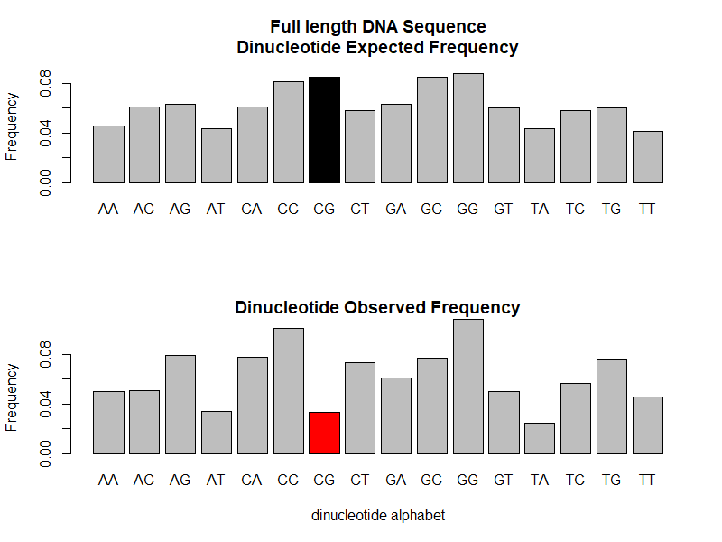
The observed frequencies for the dinucleotide alphabet are:
AA: 0.0502 CA: 0.0775 GA: 0.0611 TA: 0.0248
AC: 0.0504 CC: 0.1012 GC: 0.0773 TC: 0.0569
AG: 0.0789 CG: 0.0335 GG: 0.1082 TG: 0.0763
AT: 0.0342 CT: 0.0735 GT: 0.0503 TT: 0.0456
The comparison between observed and expected dinucleotide alphabet frequency distribution is displayed on the barplot above.
The CG dinucleotide is clearly underepresented in the full length DNA sequence as can be seen by comparing
the black and red bars. The observed frequency for CG is 0.0335 (red) while the expected frequency would be
0.0848 (black) under the assumption of a random combination of C and G following the multinomial distribution
for the single nucleotides abundance in this DNA sequence.
A \(\chi^2\) (chi-squared) test of the independence for the pairwise combination of the single nucleotides was conducted:
\(H_0\) - null hypothesis: the dinucleotides are independent combinations of two single nucleotides.
\(H_{alt}\) - alternative hypothesis: the dinucleotides are not independent combinations of two single nucleotides.
Observed \(\chi^2_{obs.}=4,669.5\,\gt\,\chi^2_{theo.}=16.9\) for the theoretical chi-squared with 9 degrees of freedom at
95%-signification level.
\(H_0\) is rejected with a p-value = 2E-16. The dinucleotides are not random combinations of two single nucleotides
and are not identically distributed. The larger discrepancy between the observed and expected frequency arises from the
CG dinucleotide (CG associates to the largest Pearson's residual).

Two CpG islands are detected in the region of the GDF15 genes (2 exons). The first detected CpG island with
our HMM algorithm has a length of 370 nt
(\(\gt 206\) as documented in the UCSC browser) harboring 29 'CG'
dinucleotides and with \(63.9\%\) C/G and is overlapping EXON 1.
The length of the sequence in the second detected CpG island is 774 nucleotides (\(\gt 600\) as documented
in the UCSC browser) harboring 85 'CG' dinucleotides and with \(68.13\%\) C/G and is overlapping EXON 2.
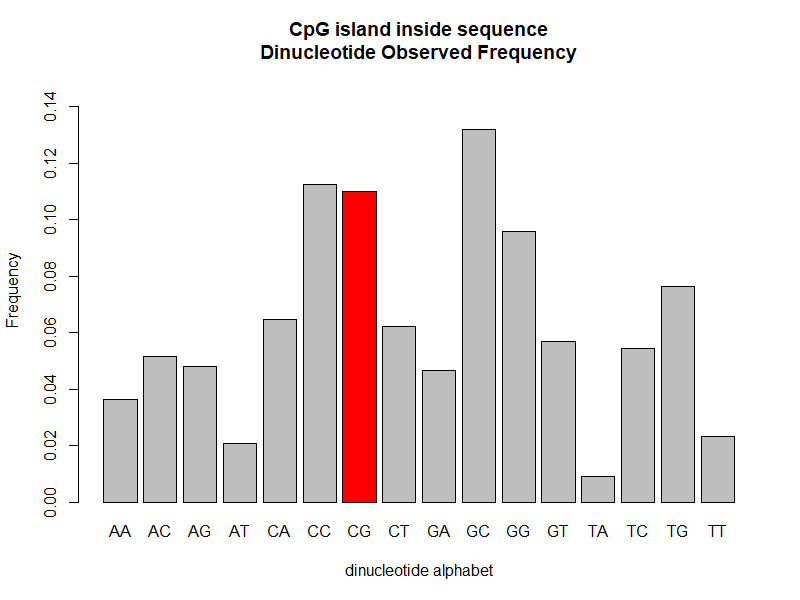
The single nucleotide observed frequencies for this second CpG island are:
A: 15.63% C: 35.01% G: 33.07% T: 16.28%
The percentage of C or G in this second CpG island sequence is
C/G: 68.08%
The observed frequencies for the dinucleotide alphabet are:
AA: 0.0362 CA: 0.0647 GA: 0.0466 TA: 0.0091
AC: 0.0517 CC: 0.1125 GC: 0.1320 TC: 0.0543
AG: 0.0479 CG: 0.1100 GG: 0.0957 TG: 0.0763
AT: 0.0207 CT: 0.0621 GT: 0.0569 TT: 0.0233
The inside CpG island dinucleotide alphabet frequency distribution is much more different than in the full DNA sequence.
We see that the CG frequency is more than threefold (\(\sim\)3.3) the CG frequency in non-CpG island regions in this case.
Our HMM parametrization allowed for the detection of the two CpG islands in the area of GDF15 that are indicated
on the UCSC browser. Our algorithm however highlighted longer CpG islands than the ones in UCSC.
The first detected CpG island is 370 nucleotides long instead of 206 (UCSC) and starts 100 nt upstream of GDF15 first exon.
The start codon 'ATG' is at position 1,191 and EXON 1 ends at 1,467. The CpG sequence spans from 1,091 to 1,460
which almost fully covers the first exon. The detected second CpG island is 774 nucleotides long instead of 600 (UCSC)
and starts 171 nt upstream of GDF15 second exon. The stop codon 'TGA' in exon 2 is at position 4,210-4,212.
The second CpG sequence spans from 3,115 to 3,888. So this CpG sequence ends 324 nt upstream of the stop codon.
It is worth noticing that the CpG island of 600 nt referenced in the UCSC
Genome browser with 65% of GC content is ending at the very same position as our second detected CpG island.
In the full length of the 64,177 nucleotides of the investigated sequence, 12 CpG islands have been detected
by our HMM algorithm that fullfill all criteria of the CpG island definition.

 In our CpG island problem, the alphabet symbols are all possible dinucleotides \(\Sigma\)= AA, CC, GG, TT, AC, AG, AT, CA, CG, CT,
GA, GC, GT, TA, TC, TG. For the sake of simplicity, we collapsed all non CG dinucleotides in the symbol 'NN', so
\(\Sigma = \) [CG, NN].