In the advanced methods of genomics, the emergence of next-generation sequencing (NGS) has created
unprecedented possibilities for the characterization of genomes and for the gene differential expression
profiling and the study of gene regulation networks and pathways. The mRNA population specifies a cell's identity and helps
to govern its present and future activities. This makes transcriptome analysis a general phenotyping method.
High-throughput mRNA sequencing (RNA-Seq) holds the promise of simulatneous transcript discovery
and abundance estimation.
In this webpage we synthetize basic knowledge infomation related to the wetlab workflow for RNA-Seq sample
preparation and sequencing. We remind ourself with the basic chemistry and most important chemical reactants
that are used routinely and how and why they are used. We recall the principles of one of the most used
sequencing platform.
Then we move to the drylab part and expose the biostatistical toolboxes which is one of the focus of our
contribution in the research program shared with our partners.
WET LAB WORKFLOW:
- Extraction, Purification and Analysis of RNA from Eukariotic cells;
- cDNA library preparation of double stranded nucleotides with blunt ends;
- Illumina Platform Sequencing;
- Coverage, depth, read lengths, counts, library size, transcript length;
- Research questions in transcriptomics: context and scope;
- Cautionary note on what RNA-Seq data are not informative of;
- Single cell scRNA-Seq or bulk RNA-Seq ?
- Other NGS ?
- Tissue expression databanks;
Total RNA Extraction, Purification and Analysis from Eukaryotic cells
Credits: Green and Sambrook. Molecular cloning, a laboratory manual. 4th edition.
ColdSpring Harbor Protocols, 2012.
A typical mammalian cell contains \(~10^{-5} \mu\)g of RNA, 80%-85% of which is ribosomal
RNA (rRNA: 28S, 18S, 5.8S and 5S species). Most of the remaining 15%-20% consists
of a variety of low molecular weight species (transfer RNAs and small snRNAs). These
abundant RNAs are of defined size and sequence and can be isolated in vitually pure form by gel
electrophoresis, density gradient centrifugation, anion-exchange chromatography or HPLC.
In contrast, messenger RNA (mRNA), which makes up between 1% and 5% of the total cellular RNA,
is heteregoneous in both size (a few hundred to many kilobases in length) and sequence.
However, most eucaryotic mRNAs carry at their 3' termini a polyadenylic acid residues tail
that is generally long enough to allow mRNAs to be purified on the basis of their affinity
to an oligo(dT) moiety. The resulting heterogeneous population of molecules collectively encodes
virtually all the polypeptides synthesized by the cell.
Because ribose residues carry hydroxyl groups in both 2' and 3' positions, RNA is chemically
much more reactive than DNA and is easily cleaved by contaminating RNases. Because RNases are
released from cells following lysis and are present on the skin, constant vigilance is required
to prevent contamination of glassware and bench tops and the creation of aerosols containing RNases.
Unfortunately, there is no simple method to inactivate RNases. Because of the presence of intrachain
disulfide bonds, many RNases are resistant to prolonged boiling and mild denaturants and are
able to refold quickly when denaturated. Unlike many DNases, RNases do not require divalent
cations for activity (like \(Mg^{2+}\)) and thus cannot be inactivated by inclusion of
ethylenediaminetetraacetic acid (EDTA) or other metal ion chelators in buffer solutions.
The best way to avoid RNases is to prevent contamination in the first place.
The key to successful purification of intact RNA from cells and tissues is speed.
It is necessary to achieve a very fast dispersal of cellular material in solution
that inactivates RNases. For this reason, very strong denaturants such as guanidinium salts are used
that simultaneously disrupt cells, solubilize their components and denature endogeneous RNases.
Guanidinium salts are chaotropic agents that destroy the 3D structure of proteins. The most powerful
chaotropic agent is guanidinium isothiocyanate (and to a lesser extent guanidinium hydrochloride) which
convert most proteins to a randomly coiled state.
Guanidinium isothiocyanate is used in the presence of a reducing agent to break protein
disulfide bonds (mercaptoethanol) and in the presence of a detergent (light anionic surfactant 'Sarkosyl',
i.e. sodium lauroyl sarcosinate) to disrupt
hydrophobic interactions. The integrity of RNA is maintained. The most recent protocol uses
monophasic lysis reagents, which contain a chaotropic agent (guanidinium isothiocyanate or
ammonium thiocyanate), acidified phenol, and a phenol solubilizer such as glycerol to enhance RNases
inactivation. After addition of chloroform (or bromochloropropane), the homogenate is separated
into aqueous and organic phases by centrifugation. RNA remains exclusively in the aqueous (upper)
phase, whereas DNA collects at the interface, and denaturated proteins are extracted into the
lower, organic phase (chloroform:phenol has a density around 1.47). RNA (single stranded) is more polar than DNA
or proteins and RNA solubilizes preferentially in water.
After recovery of the aqueous phase, RNA is precipitated by addition of isopropanol .
Commercially available monophasic lysis reagents like 'QIAzol' (QIAGEN) or 'TRIzol' (Ambion) are often used.

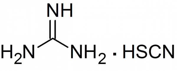

Guanidinium hydrochloride and guanidinium isothiocyanate are chaotropic agents.
DEPC : diethylpyrocarbonate is a highly alkylating agent that destroys the activity of RNases and
is used to inactivate traces of RNases that may contaminate solutions, glassware and plasticware.
The total RNA purity can be monitored by comparing relative spectrophotometric absorption spectra at 260 nm
(max absorption wavelength for nucleic acid absorption) and at 280 nm (max absorption wavelength for proteins).
Moreover, to make sure that
no DNA is contaminating the RNA sample, a RNase free DNase step can be added in the protocol, particularly
if downstream applications involve a PCR step.
Once the total RNA has been
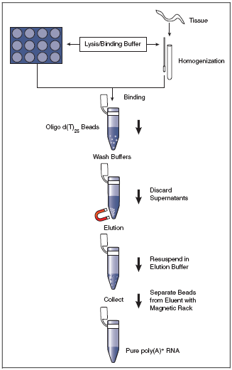
extracted and purified, mRNA is isolated from total RNA using oligo(dT) coupled to magnetic beads.
First, total RNA is dissolved in a high-salt buffer and heated briefly to 65°C-70°C, followed by
immediate cooling on ice to disrupt secondary structures. The RNA is subsequently annealed to the
oligo(dT)-magnetic beads at room temperature (see Figure to the right); the high salt binding buffer stabilizes the
poly(A)-oligo(dT) complexes. A high salt washing buffer is used to wash away unbound RNAs while retaining
oligo(dT)-bound poly(A)-mRNAs.
cDNA library preparation of double stranded nucleotides with blunt ends
The sequencing platform uses as input material dsDNA and not RNA. There are two reasons at least for that. The first is that dsDNAs are chemically generally more stable and resistant than RNAs. The second reason is that sequencing chemistry involves reactions that have been historically developped and routinely engineered on DNA.
Illumina/Solexa Platform Sequencing (2006)
Sanger dideoxy chain termination sequencing used to construct the human genome reference, was essentially
the only sequencing method used until 2005. The origins of NGS, Next Generation Sequencing technology are many
and varied. Most instruments reflect an incredible joint development of micro- or nanotechnology, organic chemistry,
optical engineering and protein engineering. Next-generation sequencing technologies share several attributes.
One attribute is the library construction step, which simply requires that DNA to be sequenced be present in relatively
short, double stranded (ds) pieces (100-800 bp) and have blunt ends. Ligation of platform-specific linker/adaptators
(synthetic dsDNA adaptators of known sequence) to the blunt-ended fragments effectively generates a library suitable
for sequencing (and there is no longer need for laborious cloning of DNA fragments into vectors and amplifying
them in bacterial hosts).
A second shared attribute is that of surface-based amplification of the library fragments.
This fragment amplification is enzymatic and occurs on a solid support (a bead or glass slide) that has covalently
linked adaptator molecules attached to its surface. These adaptators facilitate the amplification of a single fragment
into a population of fragments that provides sufficient signal from the sequencing reactions for the detection of
the incorporated nucleotides. Because each group of amplified molecules derives from a single molecule, next-generation
sequencing methods provide digital data that are indicative for a given sequence, of its abundance in the population.
Each group therefore represents a single original molecule in the library sample, and the number of
times it is read in a sequencing experiment reflects its relative frequency in the original library. This feature can
be mined in a variety of different ways during data analysis.
A third attribute is the massively parallel DNA sequencing feature; each group of amplified library fragments is
sequenced in a repeating series of steps (extension of the primer, detection of the incorporated nucleotide(s),
chemical or enzymatic scavenging of reactants or fluorescence sources) that enables all fragments to be processed
simultaneously.
A fourth hallmark of next-generation sequencing is the short read lengths that are generated relative to
former capillary sequencers, requiring use of genome-oriented bioinformatics and algorithm development.
A final attribute of next generation sequencing is the ability to generate DNA sequence
from both ends of a library fragment.
Since late 2011, there are three major platforms in common use - the Roche/454 Pyrosequencer,
the Illumina/Solexa sequencer and the Life Technologies SOLID/5550 sequencer. We focus here on the most used platform,
i.e. Illumina, and currently one of the cheapest sequencing technology which provides good quality results (small error rates).
How does Illumina platform work for DNA sequencing ?
There are plenty of very good pedagogical videos on Youtube and the reader is advised to watch them carefully
for a clear visual comprehension of the Illumina protocol.
We remind here the salient steps and features of the Illumina NGS sequencing platform.
The DNA fragments are added to a flow cell that consist of 8 microfluidic channels where the chemical reactions
are conducted and fluorescent signals are measured.
There are 4 steps:
1. SAMPLE PREP
Adaptors, i.e. known sequences of oligonucleotides, are ligated to the blunt ends of each DNA fragment in the library.
The adaptors sequences are different on the 5' end of the DNA fragment and on the 3' end. Adaptors actually encompass 3
successive sequences : from the most distal region of the fragment to the most proximal: a sequence
complementary to the flow cell oligos is ligated, than a tag sequence indexing the sample the fragment
belongs to and than a primer binding sequence.
The index tagging aims at pooling different samples in the same run to optimize the performance of the platform
(and reduce costs).
There are two types of flow cell oligos and hence two types of adaptors complementary to the flow cell oligos.
Each fragment molecule is isothermally amplified in a flow cell (generally made of 8 glass lanes). The flow cell is a grid with a lawn of possibly 400 millions oligos covalently fixed to the surface of the flow cell at one of their extremity (only one nucleotide is attached to the surface). There are up to 400 millions oligos fixed in each single lane of a flow cell. There are two types of flow cell oligos: type 1 and type 2. Type 1 is complementary to the adaptor sequence ligated on the 5'end of each DNA fragment, type 2 is complementary (and will base pair to) the adaptor sequence ligated on the 3'end of the DNA fragments in the library.
During the cluster generation step, the dsDNA of the library is denaturated and the single stranded DNAs are hybridized via their adaptators to the flow cell oligos. Then a DNA-polymerase will complete the flow cell oligo as a full double stranded DNA, using the hybridized strand as template. At the end of this step, each flow cell oligo has been elongated to the full length of the fragment that was hybridized to it. The double stranded DNA molecules in the flow cell are denaturated (with NaOH) and the complementary fragments are washed away. In the following step, the remaining ssDNAs attached to the flow cell oligo type 1 bend over and their most distal adaptator hybridize to type 2 oligos attached on the flow cell, forming bridges. Of course such bridges can also be built from ssDNA attached to oligo type 2 bending over and hybridizing to oligo type 1. DNA polymerase build the complementary fragments on each bridge producing dsDNA bridges. The dsDNA bridges are denaturated and the process is repeated over and over simultaeously for millions of clusters resulting in clonal amplifcation of all the fragments of the library.
3. SEQUENCING
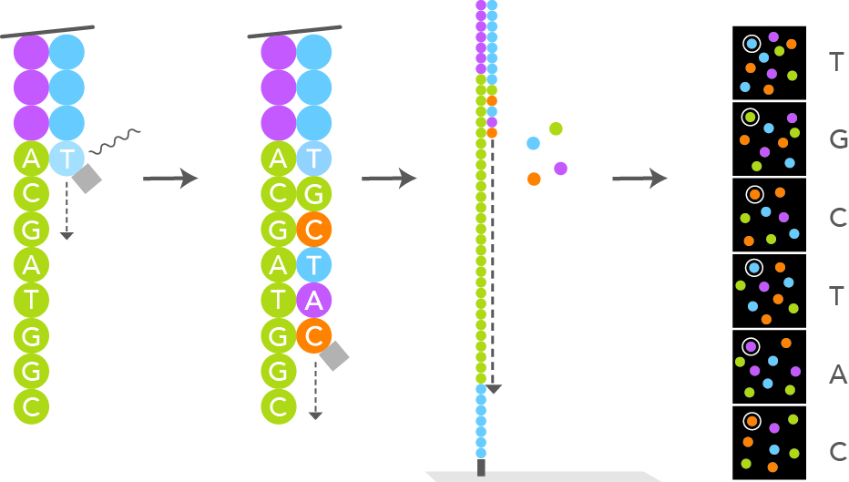
After the cluster amplification, all the reverse strands are specifically cleaved and washed off, leaving only the
forward strands. The 3'ends are distal to the plate surface and are blocked to prevent unwanted priming. The primer
sequence complementary to the primer binding site at the 3'end of the forward strand is annealed. At this moment
the sequencing by synthesis step can start. Special engineered single nucleotides are added along with the
DNA polymerase. The single nucleotide have their 3'-OH end reversibly blocked, so that the polymerization cannot procede further,
making sure that only one nucleotide at a time can be added (reversible terminator nucleotide). According to the template,
only one of the 4 different nucleotides can be added. Each particular nucleotide is also labelled with a different marker, fluorescently emitting
at a different wavelength when excited by a laser light. Each newly added nucleotide will glow differently depending on its nature (A, T, C or G) after
laser light excitation. A snapshot scan picture is taken after each new nucleotide addition step. The wavelength and intensity
of the signal is used for the base calling. The reversible terminator feature of the engineered nucleotide allows for synchronization of the laser
excitation and fluorescent signal reading of all the fragments that are simultaneously being synthetized. Once the fluorescent signals
have been recorded for all the flow cell spots,
the terminator blocking moeity of the last added nucleotide is removed, i.e. the 3'-OH end of the last desoxyribonucleotide is now made available
again for the next phosphoester binding. Hundreds of millions of clusters in the flow cell are read simultaneously in a massively
parallel process.
The number of cycles in the sequencing by synthesis determines the length of the reads.
This number is an operator chosen parameter.
After the completion of the first read, the read product is washed away from each forward strand. A complementary
primer to the index of the forward strand is annealed and further polymerized with DNA-polymerase, read, base called
and washed away. This was the completion of the first index read.
In the next step, the 3' end of the template is deprotected. The forward strand binds over and hybridizes to the second
oligo of the flow cell. Index 2 is read in the same manner as index 1. DNA polymerase then forms a double stranded
bridge. The bridge is denaturated forming two linearized strands and the 3'ends are blocked.
The forward fragment is now specifically cleaved, leaving the reverse strands attached on the second type of oligos only.
Read 2 begins with the introduction of read 2 sequencing primer. As with read 1, the sequencing by synthesis
process is conducted a number of times equal to the read length that was specified by the operator.
The determined sequences of read 2 and read 1, when matched to a reference genome, should be in the vicinity
of one another because the fragment length is smaller or equal to around 1kb max. If the read length is large and
equal to the total length of the fragment, the resulting redundancy may help resolving ambiguous alignments.
4. DATA ANALYSIS
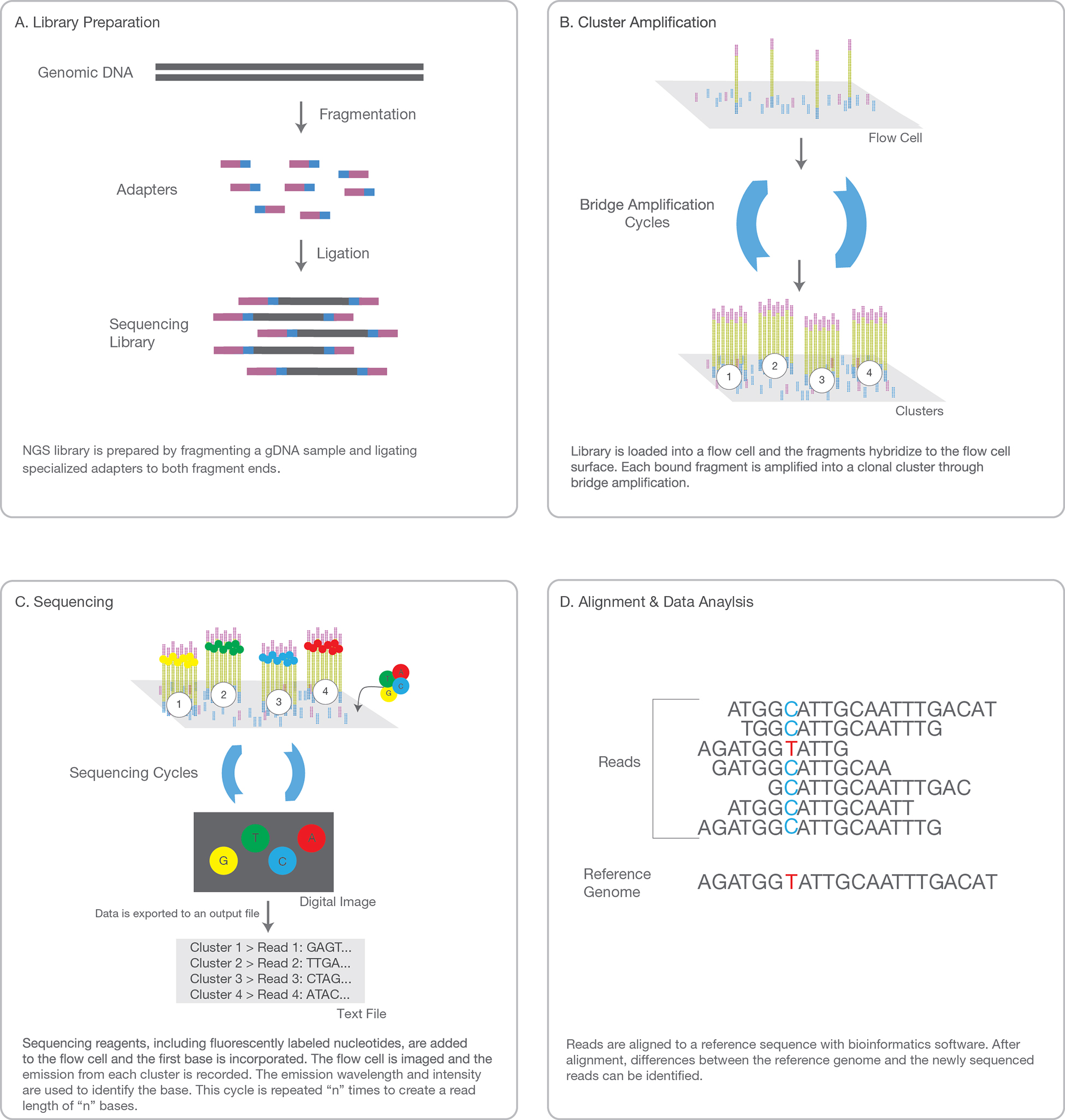
The entire sequencing process generates millions of reads representing all the fragments.
Sequences from pooled libraries are separated based on the unique indexes that were ligated to the
fragments according to the sample they belong to and introduced during the sample preparation. For
each sample forward and reverse reads are paired, creating contiguous sequences. These contiguous
sequences are aligned back to the reference genome for variant identification. The paired end information
is used to resolve ambiguous alignments.
The reads counts are normalized according to the sample
library size. The biostatistical analysis can now really start as described in the 'drylab part' below.
Coverage, depth, read length, read counts, library size, transcript length
Coverage
Next generation shotgun sequencing requires sequencing every base in a sample several times
for two reasons: first, you need multiple observations per base to achieve a reliable base
call; second, reads are not distributed evenly over an entire genome because the reads sample
the genome in a random and independent manner. Therefore, many bases will be covered by
fewer reads than the average coverage, while other bases will be covered by more reads.
This is expressed by the coverage metric, which is the number of
times a genome has been sequenced (also called the depth of sequencing). In the case
of RNA-Seq, you aim to sequence only a defined subset of an entire genome, namely the
transcriptome (the mRNA total length is around 1%-5% of the entire DNA genome). So, for RNA-Seq,
the coverage is the number of times the transcripted subset of the genome is sequenced.
Coverage calculation
In human RNA-Seq, the estimated size of the transcriptome is between 1% and 5% of the human genome size.
Given the haploid human genome is around 3.1 billion bps, the transcriptome maximal size is
around \(5\% \times 3.1 \,Gbps = 155 \,Mbps\).
In a typical RNA-Seq, the total number of reads for a sample is 20-25 million. The read length, which
is an operator defined parameter on an Illumina platform, is typically 76 bps.
The coverage \(C\) then computes:
\begin{eqnarray}
C & = & \frac{N \times L}{G} \\
& = & \frac{22\cdot 10^6 \times 76}{155\cdot 10^6} \\
& = & 10.8
\end{eqnarray}
where \(L, \,N,\, G\) are the read length (76), number of reads (22 million) and genome
subset size (155 Mbps) respectively.
Hence, the estimated average coverage of the transcriptome would be around 10-11 in this setting.
This tells us that each nucleotide (base) in the transcriptome (mRNA) of each sample has been
sequenced on average at least 10 times.
If the Illumina platform performs paired-end runs,
then the effective number of cycles is \(2\,\times\, L\, =\, 2 \times 76\,=\,152\), and
the average coverage is 20-fold in the previous setting.
Read counts and library size
The library size is the total number of reads in a sample. The reads are aligned to a reference genome
and reads are mapped to gene tags. A table is produced mapping read counts to the gene tags. For a given gene tag,
you will have the read count expressed as a mere integer number or expressed as an integer divided by the
total number of reads for that sample (CPM = Counts per million of reads).
Transcript lengths
Transcript lengths are generally not known. If you map the reads to a reference genome, it is
possible however to retrieve the transcript lengths from curated genome databases.
If the transcript lengths are known, the read counts mapped to the gene tag can be normalized
to the transcript length for that gene tag. The read counts for a given gene tag can thus also
be expressed as a number of reads divided by the transcript length of the gene tag. The unit is
then a count per kilobases (CPKB). It is known in NGS that the number of reads mapped to a particular
gene is proportional to the sequence length of that gene. So there is a bias towards longer genes.
Research questions in transcriptomics: context and scope
It is of paramount importance to clearly state the research question of your analysis at the early
beginning of the experimental setting.
Here we provide a (non-exhaustive) list of the variety of possible research questions that can be addressed through RNA-Seq
analysis:
- What are the genes that are differentially expressed for a given cell type between two or more conditions (placebo, treatment) ?
- What are the differentially expressed genes across two or more cell types (tissue 1 compared to tissue 2) ?
- What are the differentially expressed genes for a given cell type in healthy tissue compared to diseased tissue (tumoral versus healthy) ?
- What are the genes differentially expressed when a cell type is exposed to a specific growth factor ?
- How does gene expression in a given cell type change in time ?
A cautionary note on what RNA-Seq data are not informative of
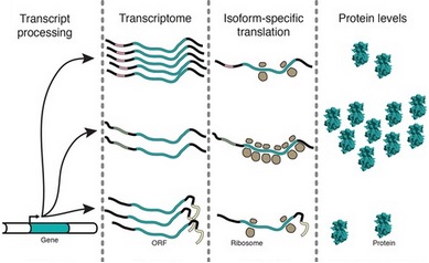
The presence of abundant transcripts is not the end of the story when protein expression is concerned.
Indeed, it is not always the case that abundant mRNA will give rise to abundant translation into proteins,
the true end point of gene expression. The correlation between mRNA and protein levels may be poor in different contexts.
In RNA-Seq, for instance, we do not measure siRNA or microRNA which will prevent mRNA to be translated properly due
to interferences.
There may exist regulation
mechanisms (repression) by which abundant mRNA will not necessarily be concordant with high protein expression levels.
There are also translation regulation mechanisms whereby the number of ribosomes active on a single mRNA are
regulated as displayed on the figure (polysome profiling) or the distribution of ribosomes or translation pausing sites and speed of
translation of a single mRNA (ribosome profiling) are regulated.
Moreover, the folding of a functional protein may require so-called chaperone proteins.
Cases are known where a protein was fully translated but was misfolded and so was not functional.
These possibilities should be kept in mind when interpreting RNA-Seq results.
Ribosome profiling (Ribo-Seq) techniques are addressing questions related to translational regulation.
Single cell scRNA-Seq or bulk RNA-Seq ?
To sequence mRNA from a single cell, one has to overcome two challenges that are not present
in standard population level (pooled cells) methods:
1) capturing single cells;
2) amplification of minute amounts of mRNA from a cell.
What is the purpose of singleRNASeq ?
The first transcriptomes generated via single-cell RNA-sequencing (scRNA-Seq) were published in 2009,
only 2 years after the first applications of RNA-seq to bulk populations of cells.
First, it is important to note that, at present, a cell type is a poorly defined concept, and we face the
question of how similar cells have to be to identify them as the same cell type.
Population (pooled cells) analysis will not reveal how a particular transcript is distributed among the cells.
Analysis of gene expression in pooled samples easily masks differences in individual cell characteristics.
Gene expression analyses in cell populations lead to the oversight of potentially important gene correlations.
Indeed, it is difficult to distinguish whether transcripts A and B are co-expressed by all cells within
the population or are separately expressed in different cell sub-types within the population. In
addition, it is also difficult to distinguish whether changes (in response to external stimulation such
as cytokines, for example) in population-level gene expression levels are due to changes in gene expression
levels in all cells in the population and or changes in the number of cells expressing particular genes.
For instance, stem cells are not necessarily always in the same state, each stem cells needs to be
analysed as an individual in order to understand the molecular mechanisms of stem cell fate decisions.
High-throughput technologies now enable the profiling of hundreds of thousands of cells in parallel,
producing an unbiased view of heterogeneity of the single cells within a population.
This type of data opens the door to several types of biological questions:
- What cell types exist within a population of cells in a particular sample? Using only scRNA-Seq data it is difficult to deduce whether observed transcriptional differences represent functionally distinct populations of cells.
- How and when cellular transitions occur and what does it tell about switches in cell state? Transitions between states can be binary or gradual, and can involve one or even multiple intermediate states. Understanding the nature of the process and possible intermediate states can lead to the identification of key genes that act as switches and drivers of these processes. Hence, clustering cells into groups on the basis of their gene expression levels is an important challenge. Can the temporal dynamic of cell transitions be understood?
- How synchronous are cell transitions in cells sampled from the same cell subpopulation?
- What can we learn about stochasticity and allele specificity of gene expression?
- How can gene-regulatory networks be constructed using gene-to-gene expression correlation and clustering of genes?
Other NGS
Third-generation sequencing is in general characterized as a single molecule sequencing and is fundamentally
different from clonal based second generation sequencing methods. Sequencing also only lasts several hours, which is very appealing
in a diagnostic setting.
The last recent development occured on two fronts:
Nanopore superlong read sequencing
Oxford Nanopore Technologies 'MinIon' sequencing is a NGS sequencing technology developped since 2014 which provides superlong reads:
5-20 Gb or even larger readlengths (25-100 Gb). Emerging long-read single-molecule sequencing technologies provide
new opportunities for detection of structural variants (SV), i.e. genomic alteration that are longer than 1kb,
like long deletion, novel sequence insertion, translocation,
mobile elements, tandem duplications, interspersed duplication, inversions, copy number variants (CNV), direct detection
of epigenetic modification, etc...
How dynamic are structural variants in humans ? It is estimated that there are 0.16 SVs (>20 bp) and 3 indels
per generation in humans. These structural variants are best investigated with long read sequencing
technologies (>20 kb) than with traditional read lengths.
Pacific Biosciences (PacBio) Single Molecule Real Time (SMRT) sequencing
Short read technologies have inherent limitations such as GC bias, difficulties mapping
to repetitive elements, trouble discriminating paralogous
sequences, and difficulties in phasing alleles.
Long read single molecule sequencers resolve
these obstacles. Moreover, they offer higher consensus
accuracies and can detect epigenetic modifications
from native DNA. The also can easily detect splicing isoforms.
Credits: Ardui et al. Single molecule real-time (SMRT) sequencing comes
of age: applications and utilities for medical
diagnostics. Nucleic Acids Research, 2018, Vol. 46, No. 5 2159–2168.
Tissue expression databanks
GTEx stands for Genotype Tissue Expression Consortium. Transcription profiles are
tissue dependent. This database provides information on transcripts ranked by tissues.
TCGA stands for The Cancer Genome Atlas.
This database provides information on transcripts ranked by tumor types.
DRY LAB BIOSTATISTICAL METHODS:
- Primary research question;
- Cross-sectional or longitudinal settings;
- Reads are count data: Poisson or not Poisson ?
- Overdispersion;
- The Negative Binomial distribution;
- Mixture distribution defined;
- The Negative Binomial and Poisson-Gamma mixture equivalence;
- The Exponential family of distributions and general linear regression models;
- Parametric and non-parametric algorithms for RNA-Seq data analysis: DESeq, DESeq2, ABSSeq, EdgeR, RUVSeq, EBSeq, baySeq, limma with voom method, NOISeq, SAMseq...
- False positives, false negatives, sensitivity (= power), specificity, variability, effect size and sample size
- Multiple testing;
- Differentially expressed gene sets interpretation: gene ontology, gene set enrichment analysis, enrichment maps, networks, pathways;
- Network inference and mechanistic modelling
Primary research questions
In RNA-Seq data, the basic outcomes we are interested in are the number of reads aligned
to a specific genome used as reference. These number of reads, counts, are a measure of the abundance
of different mRNA molecules in the cells that were sampled. The profile of mRNA expression
is tissue dependent but more importantly the differences in mRNA profiles between samples will provide
us information on differential gene expression that are dependent on the sample conditions and
settings (case or control, healthy or tumoral, drug or placebo, ...).
- What are the genes that are differentially expressed for a given cell type between two or more conditions (placebo, treatment) ?
- What are the differentially expressed genes across two or more cell types (tissue 1 compared to tissue 2) ?
- What are the differentially expressed genes for a given cell type in healthy tissue compared to diseased tissue (tumoral versus healthy) ?
- What are the genes differentially expressed when a cell type is exposed to a specific growth factor ?
- Is there a difference in gene expression profile across different cell lines when exposed to a same environment ?
- What is the difference in gene expression between a progenitor cell line and its final evolved mature state ?
- How does gene expression in a given cell type change in time ?
- How is a pool of cells from the same cell line homogeneous in gene expression ? Homogeneity and synchronocity in gene expression will require single cell RNA-seq analysis.
Cross-sectional or longitudinal settings ?
Credits: Fitzmaurice, G.M. Laird, N.M., Ware, J.H. Applied Longitudinal Analysis, Wiley, 2nd Edition, 2011.Molenberghs, G. Verbeke, G. Models for Discrete Longitudinal Data, Springer, 2005.
It can be of interest to follow the gene expression profile at different time points.
This type of analysis calls for special statistical methods known as Longitudinal Data Analysis.
When the interest is set at a fixed given common time point for two conditions, it is called
a cross-sectional study.
In Longitudinal Data Analysis, the possible correlation between different time points for a
given subject in a given condition must be taken into account and can explain part of the variance structure.
In Longitudinal Data Analysis, techniques such as GEE, Generalized Estimating Equations, are valuable to
increase precision and to better assess the significance level of the results.
Reads are counts : Poisson or not Poisson distributed ?
Poisson regression is traditionnaly conceived of as the basic count model upon
which a variety of other count models are based. The Poisson distribution may be characterized as:
$$ f(y; \,\mu) = \frac{e^{-\mu} \mu^{y_i}}{y_i !}$$
where the random variable \(y\) is the count response and parameter \(\mu\) is the mean.
Often, \(\mu\) is also called the rate or intensity parameter. Unlike most other distributions,
the Poisson distribution does not have a distinct scale parameter. Rather the scale is assumed equal to 1.
The Poisson (and negative binomial) distributions may also include an exposure
variable associated with \(\mu\).
The variable \(t\) is considered to be the length of time or length in space, or the area or the volume of space
during or in which events or counts occur. This is typically called the exposure. If \(t=1\), then the
Poisson probability distribution reduces to the standard form. If \(t\) is constant, or varies between
events, then the distribution can be parametrized as:
$$ f(y; \,\mu) = \frac{e^{-t_i\mu_i} (t_i\mu_i)^{y_i}}{y_i !}$$
The rate at which events occur in a period of time or length in space is \(\mu\), with a probability
of occurence being \(\mu\) times the length of the period or size of the space length or area or volume.
A unique feature of the Poisson distribution is the relationship of its mean to the variance:
they are equal. This is termed equidispersion. The fact that it is rarely found
in real data has driven the development of more general count models, which do not assume such
a restrictive relationship between the mean and the variance of the distribution.
Poisson counts, y, are examples of a Poisson process. Each event in a given time period
or space length, area or space volume, that is subject to the counting process is independent of one
another; they enter into each period or area or length in space according to a uniform distribution.
The fact that they are \(y\) events in region A has no bearing on how many events are counted in region B.
This assumption may be violated in RNA-Seq data because some transcripts are co-expressed and could be
underpinned by a common signalling or transcription pathway.
The Poisson model carries with it various assumptions in addition of those given above.
Violations of Poisson assumptions usually result in oversdispersion, i.e. the variance
is significantly larger than the mean.
Violations of equidispersion indicate correlation in the data, which affects standard errors of the parameter
estimates. Model fit is also affected. A simple example of how distributional assumptions may be
violated is the following. Given a Poisson distribution having a mean of 2, some 13/% of the outcome are predicted
to be zero. If, in fact, we are given an otherwise Poisson distribution having a mean of 2, but with 50/% of zeros,
it is clear that the Poisson distribution may not adequately describe the data at hand.
Modifications should be made to the Poisson model to account for discrepancies in the goodness of fit
of the underlying distribution: zero-inflated Poisson or zero-truncated Poisson directly address such problems.
This also applies to the negative binomial distribution.
Overdispersion
Credits: Hilbe, J.M. Negative Binomial Regression. Cambridge University Press, 2nd Edition, 2011. Few real-life Poisson data sets are truly equidispersed. Overdispersion to some degree is inherent
to the vast majority of Poisson data. Although rarely discussed, negative binomial (NB2) models may
also be overdispersed. We may define negative binomial overdispersion as occuring when calculated
model variance exceeds \(\mu\,+\,\alpha\mu^2\). That is a count model may be both Poisson and negative
binomial overdispersed if the variance produced by the estimated model exceeds the nominal negative binomial variance.
A model can also be Poisson overdispersed and negative bionomial underdispersed or equidispered.
How can we know ? By observing the negative binomial (NB2) Pearson dispersion.
Not all overdispersion is real. Apparent overdispersion may sometimes be identified and the model amended to eliminate
it. First, we address the difference between real and apparent overdispersion and what can be done about the latter.
1. What is overdispersion ?
Overdispersion in Poisson models occurs when the response variance is greater than the mean.
2. What causes overdispersion ?
Overdispersion is caused by positive correlation between responses or by an excess variation
between response probabilities or counts. Overdispersion also arises when there are violations in
the distributionals of the data, such as when the data are clustered and thereby violate the likelihood
independence of observations assumption.
3. Why is overdispersion a problem ?
Overdispersion may cause standard errors of the estimates to be deflated or underestimated, i.e. a variable may
appear to be a significant predictor when it is in fact not significant.
4. How is overdispersion recognized ?
A model may be overdispersed if the value of the Pearson (or \(\chi^2\)) statistic divided by the degrees of freedom
(dof) is greater than 1.0. The quotient of either is called the dispersion. Small amounts of overdispersion are
of little concern; however, if the dispersion statistic is greater than 1.25 for moderate sized models, then a correction
may be warranted. Models with large numbers of observations may be overdispersed with a dispersion statistic of 1.05.
5. What is apparent overdispersion; how may it be corrected ?
Apparent overdispersion occurs when:
- the model omits important explanatory predictors;
- the data include outliers;
- the model fails to include a sufficient number of interaction terms;
- a predictor needs to be transformed to another scale;
- the link function is misspecified: the assumed linear relationship between the response and the link function and predictors is mistaken;
The Negative Binomial distribution
The negative binomial distribution allows modeling of a wide range of count response situations (like reads counts in RNA-Seq data). Recall that Poisson distributions have the major assumption of equidispersion (i.e. mean = variance). The negative bionomial allows extra variation:
- a quadratic adjustment of the variance function \(\mu\,+\,\alpha\mu^2\) (this is the NB2 variance function where 2 refers to the quadratic term). \(\alpha\) in the previous fromula is called the negative binomial heterogeneity parameter or the overdispersion parameter. The variance is always larger than the mean and accomodates for the overdispersion a Poisson model would suffer.
- a modification to the NB2 probability distribution, resulting in an amended log-likelihood function.
When the negative binomial PDF is understood within the context of GLM (Generalized Linear Models), it should be thought of as being characterized as the probability of successes and failures in a series of independent and identical Bernoulli trials. Specifically, the PDF underlying the GLM-based negative binomial model is based on the distribution of \(y\) failures before the \(r^{th}\) success occurs in a series of Bernoulli trials. In this parametrization, both \(r\) and \(y\) are integers. When \(r\) is limited to integer-only values, the distribution is termed a Pascal distribution. When \(r\) is allowed to take any positive real value, the distribution is known as a Polya distribution. Both forms are a special case of the more general negative binomial distribution.
Suppose you were interested in the number of failures \(y\) before the realization of the \(r^{th}\) success in a series of Bernoulli trials (for which each individual outcome is binary). What is the probability distribution of the random variate \(Y=y\), given that the probability of success for an indivual outcome is \(p\)?
The last trial would give a success as an outcome. Before the last outcome, you would have \(r-1\) successes and \(y\) failures. There are many ways to have a sequence of \(r-1\) sucesses and \(y\) failures: the number of such ways is calculated from combinatory analysis and writes: $$ \displaystyle{r+y-1 \choose r-1 } = \frac{(r+y-1)\,!}{(r-1)\,!\,\,y\,!} $$ which also equals to $$ \displaystyle{r+y-1 \choose y } = \frac{(r+y-1)\,!}{(r-1)\,!\,\,y\,!} $$ Hence, the probability to observe exactly \(y\) failures before the \(r^{th}\) success is: $$ P(Y=y) = b^*(y;\,p, r) = \displaystyle{r+y-1 \choose r-1 } p^{r}\,(1-p)^y $$ This is the classical derivation of the Pascal ditribution (Negative Binomial distribution, also noted \(b^*(y;\,p, r)\)).The mean and the variance of the Negative Binomial distribution are: \begin{eqnarray} E[Y] = \mu & = & r\,\frac{1-p}{p}\\ Var[Y] & = & r\,\frac{1-p}{p^2} \end{eqnarray}
How can we relate \(p\) to the heterogeneity parameter in the variance function?
Dividing the variance by the mean from the above formula gives:
\begin{eqnarray}
\frac{Var[Y]}{E[Y]} & = & \frac{1}{p} \\
& = & \frac{\mu + \alpha\mu^2}{\mu} \\
& = & 1 + \alpha\mu
\end{eqnarray}
and equating the first line with the last one gives:
$$ p = \frac{1}{1+\alpha\mu}$$
where the probability of success \(p\) is related to the mean \(\mu\) and the heterogeneity
parameter \(\alpha\) (overdispersion parameter).
How can we relate \(r\) (number of successes) to the heterogeneity parameter?
Now that \(p\) is related to \(\mu\) and \(\alpha\), we can use the expression of the mean of
the negative binomial distribution to write:
\begin{eqnarray}
\mu & = & r\frac{1-p}{p} \\
& = & r\frac{1-\frac{1}{1+\alpha\mu}}{\frac{1}{1+\alpha\mu}} \\
& = & r\,\alpha\mu
\end{eqnarray}
Hence, it holds that $$ r\cdot \alpha = 1$$ and \(r=\frac{1}{\alpha}\).
\(r\) is the inverse of the heterogeneity parameter. \(r\) is indeed inverseley related to overdispersion.
Note that if \(r\) is integer, then \(\alpha\) would be integer rational.
Allowing \(r\) to be positive real gives more pliability to the model. As actually employed in a statistical model,
\(r\) indicates the amount of excess correlation in the data. Limiting it to integer values
would dismiss the continuous nature of the range of correlation in data.
The point here is that the negative binomial statistical model is not based on a single derivation. It can be derived
as Poisson-Gamma mixture (see below), as a series of Bernoulli trials as just shown, as a Polya-Eggenberger
urn model or as a type of inverse binomial distribution.
Note also that the geometric is a variety of negative binomial (with \(\alpha=1\)).
If \(\alpha=0\), then it is a Poisson distribution but \(\alpha\) can only approach zero, never reach it.
If \(\alpha\) is close to zero, it is statistically indistinguishable from a Poisson model.
Mixture distribution defined
Credits: Rizzo, M.L. Statistical Computing with R. Chapman & Hall, 2008.What is a mixture distribution ? It should not be confused with convolution (the
probability distribution function, PDF of \(S\), a random variable
that is the sum \(S=X_1 + X_2\) of two independent random variables, \(X_1\) and \(X_2\), each with probability distribution
function PDF1 and PDF2, is the convolution product of PDF1 with PDF2).
Instead, a mixture distribution is a weighted sum of two PDFs such that the
resulting PDF be normalized to one.
More formally, we can successively define the discrete mixture distribution of a sequence of discrete random
variables and the mixture distribution of a sequence of continuous random variables.
A random variable \(X\) is a discrete mixture if the distribution of
\(X\) is a weighted sum \(F_X(x) = \sum \theta_i\,F_{X_i}(x)\) for some sequence of random variables
\(X_1, X_2, \cdots \) and \(\theta_i \gt 0\) such that \(\sum_i \theta_i = 1\).
The constants \(\theta_i\) are called the mixing weights or mixing probabilities.
A random variable \(X\) is a continuous mixture if the distribution of \(X\) is
\(F_X(x) = \int_{-\infty}^{\infty}F_{X|Y=y}(x)f_Y(y)\,dy\) for a family \(X|Y=y\) indexed
by the real numbers \(y\) and weighting functions \(f_Y\) such that \(\int_{-\infty}^{\infty} f_Y(y)\, dy = 1\).
The Negative Binomial and Poisson-Gamma mixture equivalence
Credits: Hilbe, J.M. Negative Binomial Regression. Cambridge University Press, 2nd Edition, 2011.
Let us first recall the Gamma distribution. The Gamma ditribution is the probability density of a continuous random
variable, with positive real values only, which has the form:
$$ \Gamma(x;\,\alpha, \beta) = \frac{1}{\Gamma(\alpha)\,\beta^{\alpha}}x^{\alpha-1}\cdot e^{-\frac{x}{\beta}}$$
The mean is \( \mu= \alpha\,\beta\), the variance is \(\sigma^2 = \alpha\,\beta^2\).
If \(\alpha=1\), the Gamma distribution reduces to the exponential distribution. With integers \(\alpha\), the
Gamma distribution is equivalent to a sum of \(\alpha\) exponential distributions
(a convolution of exponential distributions yields a Gamma distribution).
But of course, in full generality,
\(\alpha\) is not restricted to integers and can take any real positive value.
Our point here is to show that a discrete random variable with a negative binomial distribution is
mathematically a special case of a Poisson-Gamma continuous mixture random variable .
The interesting useful attribute here of the Poisson-Gamma mixture random variable is that it accomodates
overdispersion or correlated Poisson counts in real experimental settings of biological interests.
We start with a Poisson distribution araising from a count (digital) outcome characterized by:
$$ f(y;\,\lambda, u) = \frac{e^{-\lambda_i u_i}\cdot(\lambda_i\cdot u_i)^{y_i}}{y_i !}$$
This distribution can be thought of as a Poisson model with Gamma heterogeneity where the Gamma noise has a mean of 1.
Stated otherwise, the Poisson distribution has a \(\lambda\) rate per unit of time \(u\) (or unit of length or
area or volume) which is itself a random variable that is Gamma distributed with the constraint that \(u\) has its mean
equals to one.
Explicitely, with the fullfilment of obeying the definition of a continuous mixture given above, we can write:
Definition of a mixture:
A random variable \(Y\) is a continuous mixture if the distribution of \(Y\) is
\(F_Y(y) = \int_{-\infty}^{\infty}F_{Y|U=u}(y)f_U(u)\,du\) for a family \(Y|U=u\) indexed
by the real numbers \(u_i\) and weighting functions \(f_U\) such that \(\int_{-\infty}^{\infty} f_U(u)\, du = 1\).
We have for the weighting function:
$$ f_U(u) = \frac{\nu^{\nu}}{\Gamma(\nu)}u^{\nu-1}\cdot e^{-\nu\, u}$$
which is a particular Gamma distribution
whose integral is equal to 1 by definition of a distribution, and with \(\alpha=\nu\) and \(\beta=\frac{1}{\nu}\),
so with mean \(=\alpha\cdot\beta = \nu\cdot\frac{1}{\nu} = 1\). The mean noise of U is equal to 1.
The distribution of \(Y\), conditionned on U=u, is a Poisson distribution:
$$ F_{Y|U=u}(y) = \frac{e^{-\lambda_i u_i}\cdot(\lambda_i\cdot u_i)^{y_i}}{y_i !}$$
As a result, the unconditional distribution of \(Y\), or the Poisson-Gamma mixture distribution, is derived from the following expression:
\begin{eqnarray}
F_Y(y; \lambda, \nu) & = & \int_{-\infty}^{\infty}F_{Y|U=u}(y)f_U(u)\,du \\
& = & \int_{0}^{\infty} \frac{e^{-\lambda_i u_i}\cdot(\lambda_i\cdot u_i)^{y_i}}{y_i !}\, \frac{\nu^{\nu}}{\Gamma(\nu)}u^{\nu-1}\cdot e^{-\nu\, u}\,du \\
& = & \frac{\lambda_i^{y_i}}{\Gamma(y_1 + 1)}\frac{\nu^{\nu}}{\Gamma(\nu)}\,\int_0^{\infty}e^{-(\lambda_i+\nu)u_i}\cdot u_i^{y_i + \nu - 1}\,du_i\\
& = & \frac{\lambda_i^{y_i}}{\Gamma(y_1 + 1)}\frac{\nu^{\nu}}{\Gamma(\nu)}\,\color{blue}{\frac{\Gamma(y_i+\nu)}{(\lambda_i+\nu)^{y_i+\nu}}}\underbrace{\int_0^{\infty} \color{blue}{\frac{(\lambda_i+\nu)^{y_i+\nu}}{\Gamma(y_i + \nu)}} \, e^{-(\lambda_i+\nu)u_i}\cdot u_i^{y_i+\nu-1}\,du_i}_{=1}\\
& = & \frac{\Gamma(y_i+\nu)}{\Gamma(y_1 + 1)}\frac{1}{\Gamma(\nu)}\,\frac{\nu^{\nu}\cdot\lambda_i^{y_i}}{(\lambda_i+\nu)^{y_i+\nu}}\\
& = & \frac{\Gamma(y_i+\nu)}{\Gamma(y_1 + 1)}\frac{1}{\Gamma(\nu)}\,\frac{\nu^{\nu}}{(\nu+\lambda_i)^{\nu}}\cdot\frac{\lambda_i^{y_i}}{(\nu+\lambda_i)^{y_i}}\\
& = & \frac{\Gamma(y_i+\nu)}{\Gamma(y_1 + 1)}\frac{1}{\Gamma(\nu)}\,\Big(\frac{\nu}{\nu+\lambda_i}\Big)^{\nu}\cdot \Big(\frac{\lambda_i}{\nu+\lambda_i}\Big)^{y_i}
\end{eqnarray}
In the first parenthesis, we divide both the numerator and denumerator by \(\nu\). The second parenthesis writes:
$$ \frac{\lambda_i}{\nu+\lambda_i} = \frac{\nu + \lambda_i - \nu}{\nu+\lambda_i} = 1-\frac{\nu}{\nu+\lambda_i}=1-\frac{1}{1+\frac{\lambda_i}{\nu}}$$
Hence,
\begin{eqnarray}
F_Y(y; \lambda, \nu) & = & \frac{\Gamma(y_i+\nu)}{\Gamma(y_1 + 1)}\frac{1}{\Gamma(\nu)}\,\Big(\frac{1}{1+\frac{\lambda_i}{\nu}}\Big)^{\nu} \, \Big(1-\frac{1}{1+\frac{\lambda_i}{\nu}}\Big)^{y_i}
\end{eqnarray}
Inverting \(\nu\), the Gamma scale parameter, yields \(\alpha=\frac{1}{\nu}\), which is the negative binomial heterogeneity
or overdispersion parameter. We also substitute \(\mu_i=\lambda_i\) and we will promptly recognize the resulting Negative
Binomial probability mass function:
\begin{eqnarray}
f(y; \mu, \alpha) & = & \frac{\Gamma(y_i+\frac{1}{\alpha})}{\Gamma(y_i+1)\Gamma(\frac{1}{\alpha})}\cdot \Big(\frac{1}{1+\alpha\mu_i}\Big)^{\frac{1}{\alpha}}\Big(1-\frac{1}{1+\alpha\mu_i}\Big)^{y_i}\\
& = & \left(\begin{array}{c}y_i+\frac{1}{\alpha}-1 \\ \frac{1}{\alpha}-1\end{array}\right)\,\Big(\frac{1}{1+\alpha\mu_i}\Big)^{\frac{1}{\alpha}}\Big(1-\frac{1}{1+\alpha\mu_i}\Big)^{y_i}\\
& = & b^*(y_i;\,p, k)
\end{eqnarray}
where \(b^*(y_i;\,p, k)\) is the short notation for the negative binomial random variable associated to a sequence
of independent Bernoulli trials with probability of success equals to \(p=\frac{1}{1+\alpha\mu_i}\) and which gives the probability of observing \(y_i\) failures
before the \(k^{th}\) success is achieved, and where \(k=\frac{1}{\alpha}=\nu\). In this Negative Binomial context, both \(y_i\) and \(k\) are integers.
The total number of trials is \(y_i + k\).
The Exponential family of distributions and the general linear model for regression
Credits: Hilbe, J.M. Negative Binomial Regression. Cambridge University Press, 2nd Edition, 2011.Fitzmaurice, G.M. Laird, N.M., Ware, J.H. Applied Longitudinal Analysis, Wiley, 2nd Edition, 2011.
Molenberghs, G. Verbeke, G. Models for Discrete Longitudinal Data, Springer, 2005.
Generalized linear models are a broad class of regression models suitable for analyzing diverse types of univariate responses, e.g. continuous, binary, counts. A generalized linear model for \(Y_i\) has a three-part specification:
- a distributional assumption
- a systematic component which specifies the effects of the covariates, \(X_i\), on the mean of the distribution of \(Y_i\), and which can be expressed via a 'linear' predictor: \(\eta_i=\sum_{k=1}^{p}\beta_k\,X_{ik}\) where \(\eta_i\) is linear in the regression parameters.
- a link function
The motivation for describing a distribution as a particular member of the exponential family is three fold:
1) We want to demonstrate that probability distributions for seemingly quite different data type (continuous, binary, count data) have much in common as members of the family.
2) We want to emphasize the importance of the canonical "location" parameter in exponential family distributions; the canonical location parameter is closely related to, but generally not equal to, the mean of the distribution.
3) We want to emphasize that the variance of many exponential family distributions depends on the mean, via the so-called variance function.
All distributions that belong to the exponential family can be expressed as follows: \begin{equation} f(y_i; \theta_i, \phi) = exp\Big[\frac{y_i\theta_i\, -\, b(\theta_i)}{\phi} + c(y_i; \phi)\Big] \end{equation} where
- \(\theta_i\) is the canonical location parameter (related to the mean) or link function
- \(b(\theta_i)\) is the cumulant
- \(\phi\) is the scale parameter, set to one in discrete and count models
- \(c(y_i; \phi)\) is the normalization term, guaranteeing that the probability function sums to unity.
The exponential family form is unique in that the first and second derivative of the cumulant,
with respect to \(\theta\), produce the mean and variance functions respectively. The important point to
remember is that if one can convert a probability function into exponential family form, its unique
properties can be easily used to calculate the mean and variance, as well as facilitate estimation of parameter
estimates based on the distribution. All members of the class of generalized linear models can be converted
to exponential form, with
\begin{eqnarray}
b^{\prime}(\theta_i) & = & mean \\
b''(\theta_i) & = & variance
\end{eqnarray}
One sometimes starts from specifying a mean and variance function:
\begin{eqnarray}
E[Y] & = & \mu \\
Var[Y] & = & \phi \cdot v(\mu)
\end{eqnarray}
The variance function is related to a particuliar member of the exponential family
(and parameters can be estimated using maximum likelihood principles).
In the case of the Gaussian (normal) distribution, we have:
- \(\theta_i = \mu_i\)
- \(b(\theta_i) = \frac{\mu_i^2}{2}\)
- \(\phi = \sigma^2\)
- \(c(y_i;\phi) = -\frac{1}{2}\big[\frac{y_i^2}{\sigma^2}+ln(2\pi\sigma^2)\Big]\)
In the case of the binomial distribution, we have:
- \(\theta_i = ln \frac{\mu_i}{1-\mu_i} = logit(\mu_i)\)
- \(\phi = 1\)
- \(b(\theta_i)=-ln(1-\frac{exp(\theta_i)}{exp(1+\theta_i)})\)
In the case of the Poisson distribution, we have:
- \(\theta_i = ln\, \mu_i\)
- \(\phi = 1\)
- \(b(\theta_i)=\mu_i\)
Finally, in the case of the negative binomial distribution, we have: $$ f(y_i; \theta_i, \phi) = exp\Big[\frac{y_i\theta_i\, -\, b(\theta_i)}{\phi} + c(y_i; \phi)\Big] $$ $$ f(y_i; \theta_i, \phi) = \frac{(y_i+r-1)\,!}{y_i\,!\,(r-1)\,!}p_i^r\, (1-p_i)^{y_i}$$ $$ f(y_i; \theta_i, \phi) = exp\Big[y_i\,\underbrace{ln(1-p_i)}_{\color{red}{LINK}}+\underbrace{r\, ln\,p_i}_{\color{red}{CUMULANT}} + ln\Big(\frac{(y_i+r-1)\,!}{y_i\,!\,(r-1)\,!}\Big)\Big]$$
- \(\theta_i = ln\,(1-p_i)\)
- \(\phi = 1\)
- \(b(\theta_i)=-r\,ln\,p_i = -r\,ln\,(1-exp(\theta_i))=-\frac{1}{\alpha}ln\,\frac{1}{1+\alpha\,\mu_i}=\frac{1}{\alpha}ln\,(1+\alpha\,\mu_i)\)
Parametric and non-parametric algorithms for RNA-Seq data analysis: DESeq, DESeq2, ABSSeq, EdgeR, RUVSeq, EBSeq, baySeq, limma with voom transformation, NOISeq, SAMseq...
Credits:
Rapaport, F. et al. (2013) Comprehensive evaluation of differential expression analysis methods for RNA-seq data.
Genome Biology, 14(9):R95.
A basic task in the analysis of count data from RNA-seq is the detection of differentially expressed genes.
The count data are presented as a table which reports, for each sample, the number of sequence fragments
that have been assigned to each gene, reflecting the abundance of transcripts.
An important analysis question is the quantification and statistical inference of systematic changes between
conditions, as compared to within-condition variability.
There are parametric biostatistical methods, Bayesian methods and non-parametric methods. A variety of R packages
implementing the statistical algorithms are available on Bioconductor R.
We review here some of the most used packages for RNAseq analysis in R and their salient features.
No single method consistently outperforms the others but there are significant differences among the methods.
It should be emphasized that increasing the number of replicate samples provides significantly more detection
power than increased sequencing depth.
1. PARAMETRIC METHODS
Among the parametric methods the two most commonly used are DESeq (or DESeq2) and edgeR; both methods showing good
ROC curve performances as compared to other methods. EdgeR appears to be a bit less conservative than DESeq, meaning
that EdgeR has a higher true positive rate (TPR) than DESeq, but this is often at the cost of a poorer false positive rate (FPR).
DESeq is still more conservative (robust) to outliers while edgeR becomes more liberal
when outliers are introduced. Rappaort et al. showed however, in their paper, that null model evaluation of type I error was better
for EdgeR than for DESeq. The computational time is higher with DESeq when sample size is increased while edgeR has its
computational time rather independent on sample size. Both DEseq and EdgeR use the Negative Binomial distribution as the
statistical model for the reads counts.
The main differences in the statistical methods implemented both
in DEseq and EdgeR concern the normalization method used for library size correction and the way the dispersion factor
(a.k.a. heterogeneity parameter) is estimated.
1) DESeq and DESeq2
Credits:
Love, M.I., Huber, W., Anders, S. (2014) Moderated estimation of fold change and dispersion for RNA-seq data with DESeq2.
Genome Biology, 15:550. 10.1186/s13059-014-0550-8
The package DESeq2 provides methods to test for differential expression by use of negative binomial generalized
linear models; the estimates of dispersion and logarithmic fold changes incorporate data-driven prior distributions.
Input data (un-normalized counts)
As input, the DESeq2 package expects count data as obtained, e.g., from RNA-seq or another high-throughput
sequencing experiment, in the form of a matrix of integer values. The value in the i-th row and the j-th column
of the matrix tells how many reads can be assigned to gene i in sample j. Analogously, for other types of assays,
the rows of the matrix might correspond e.g. to binding regions (with ChIP-Seq) or peptide sequences (with
quantitative mass spectrometry).
The values in the matrix should be un-normalized counts or estimated counts of sequencing reads
(for single-end RNA-seq) or fragments (for paired-end RNA-seq). The RNA-seq workflow describes multiple techniques
for preparing such count matrices. It is important to provide count matrices as input for DESeq2’s statistical
model (Love, Huber, and Anders 2014) to hold, as only the count values allow assessing the measurement
precision correctly. The DESeq2 model internally corrects for library size, so transformed or normalized
values such as counts scaled by library size should not be used as input.
The method used in DESeq to compute the scaling factor to correct for the library size is the
geometric mean method. DESeq computes a scaling factor for a given sample by computing
the median of the ratio, for each gene, of its read count over its geometric mean across all samples. It
then uses the assumption that most genes are not DE and uses this median of ratios to obtain the scaling
factor associated with this sample.
DESeq estimates \(\alpha\), the heterogeneity parameter (dispersion factor), by breaking the variance
estimate to a combination of the Poisson estimate (i.e. the mean expression of the gene) and a second
term which models the biological expression variability.The detailed variance estimation method is
documented in this DESeq2 article.
2) EdgeR
Credits: Chen, Y. Robinson,M. et al. edgeR: differential expression analysis
of digital gene expression data. User's Guide. R vignette, 2016.
The method used in EdgeR to compute the scaling factor to correct for the library size is the
TMM (Trimmed Mean of M values or Trimmed Mean of the log expression ratios) as
detailed in this TMM article.
The TMM computes a scaling factor between two experiments by using the weighted average of subset of
genes after excluding genes that exhibit high average coverage and genes that have large differences in expression.
EdgeR estimates \(\alpha\), the heterogeneity parameter (dispersion factor), as a weighted combination
of two components. The first is a gene specific dispersion effect and the second is a common dispersion
effect calculated from all genes. The detailed estimation method is documented in edgeR vignette:
edgeR Users Guide.
3) ABSSeq
Credits:
Wentao Yang, Philip C. Rosenstiel and Hinrich Schulenburg (2016) ABSSeq: a new RNA-Seq analysis method based on modelling absolute expression differences.
BMC Genomics, 17:541.
ABSSeq uses a negative binomial distribution to model absolute expression differences between conditions, taking
into account variations across genes and samples as well as magnitude of differences. In comparison to other methods,
ABSSeq shows higher performance on controlling type I error rate but is much more conservative in finding true positives.
ABSSeq infers differential expression directly by the counts difference between conditions. It
assumes that the sum counts difference between conditions follow a Negative Binomial distribution with mean \(\mu\)
(proportional to expression level) and dispersion factor \(r\) (inverse of dispersion heterogeneity parameter \(\alpha\)).
The \(\mu\) and \(r\) depend on variations in the experiment, i.e., biological variations (biological replicates), sequencing
and mapping biases. Typically, the number of replicates in a study is small and not enough to reveal all the variations.
To overcome this problem, a common solution is to borrow information across genes. A local regression
to smooth dispersion across genes is used. The smoothed dispersions are then used to produce pseudocounts in the
\(\mu\) estimation to account for dynamic dispersions across expression levels, which in turn moderates the
fold change.
The method used in ABSSeq to compute the scaling factors to correct for the library size is either the
TMM (Trimmed Mean of M values), from EdgeR or geometric mean , from DESeq,
or quantile by reads count in the first three quartiles, from baySeq, or
total reads count , or even user defined scaling factors.
The shortcoming of ABSeq is that it is difficult to compare the results with other methods based on fold changes
rather than on absolute difference in gene expression abundances.
2. TRANSFORMATION APPROACH METHODS
voom+limma
3. BAYESIAN APPROACH METHODS
EBSeq
False positives, false negatives, sensitivity, specificity, variability, effect size and sample size
It is of paramount importance to make sure that the statistical design of your RNA-seq experimental setting
has been made BEFORE you start your experiments.
In RNA-seq data, you will deal with a number of null hypotheses, \(H_0\), that there is no
differential expression for a given gene across two conditions. The alternative hypotheses being
that there is a differential gene expression across the conditions.
You either accept or reject the null hypothesis.
There are two problematic conclusions when conducting a statistical test:
- you reject the null hypothesis wrongly : you reject the null when the null is actually true. This means you found false positives. The probability to reject the null given it is actually true is called \(\alpha\) or the type I error.
- you accept the null hypothesis wrongly : you accept the null when the null is actually false (the alternative is true). This means you found false negatives. The probability to accept the null given it is actually false is called \(\beta\) or type II error.
Similarly, \(1-\alpha\) is called the specificity , it is the probability to accept the null when the null is true (or the probability to find the true negatives).
The fundamental statistical concerns are to relate 4 concepts in order to determine the sample size in your experimental design:
- What is the inherent variability of the gene expression profiles in the different conditions ? Most often, you don't know it. But you need to get some initial indication of the variance in your data. To have an initial estimation, you should consider to conduct pilot trials or explore previous literature. You need to have an initial estimate of the variance, \(\sigma^2\), of the gene expression level between any biological replicates in the different conditions or at least for the control condition.
- What risk do you accept for false positives ? This is the famous type I error (\(\alpha\)). You most often set \(\alpha = 0.05\) (or = 0.01) upfront. This \(\alpha\) is the conditional probability to reject the null hypothesis given that it is actualy true.
- What is the measure of a success for a differentially expressed gene ? What is the fold change you would be happy to detect ? This is the famous effect size, \(\delta\). If there is truly an effect between your conditions (control and case), what is the threshold size in the difference between the cases and the control that you would be happy to detect. In RNA-seq data, the effect size is the fold change threshold that would be considered relevant to detect. You must accept that you would not be interested in genes for which the fold change is smaller than the effect size you fixed before starting the experiment.
- What power do you want to achieve ? If there is truly an effect (if there is truly a difference in gene expression across conditions and this effect is larger or equal to the effect size you expect), what are the chances that your experimental setting will detect the effect ? You have to fix the power before you carry out your experiments. The power is \(1-\beta\). So fixing \(\beta\) is equivalent to fixing the power.
Can you reduce \(\alpha\) and increase the power simultaneously (or equivalently reduce simultaneously type I error and type II error) ? The answer is no. There is a trade-off to accept. For a given effect size and a given sample size, if you want to decrease the type I error, you will increase the type II error (and decrease the power) and reciprocally. There is no free lunch.
As a general rule of thumb, to determine the sample size for your experimental setting, take \(\alpha\) = 0.01 or 0.05, \(\beta\) = 0.10 or 0.20 (power of 90% or 80%), to detect an effect if there is truly one.
In the following, we provide an illustration of the sample size determination for the number
of biological replicates in case versus control for a differential gene expression effect size equal to a fold
change of 2 across two conditions applied to a human lymphatic endothelial cell line. The reads counts for any
single gene are assumed to
follow a negative binomial distribution with the same heterogeneity parameter across conditions. Pilot results showed that the
heterogeneity parameter in the read counts in the control condition is rarely larger than 0.05 when the
number of reads is larger than 1000. We want to fix the type I error for a single gene to 0.01.
We would like to calculate the sample size (the number of biological replicates)
to achieve a power of 0.90 to detect differentially expressed genes across the conditions.
Equivalently, for a sample size of 3 (or 4) in each condition, what is the power we can achieve for an
effect size set to a fold change of 2 (or log2 fold change = 1), if \(\alpha\)=0.01 and the heterogeneity
parameter is around 0.05 ?
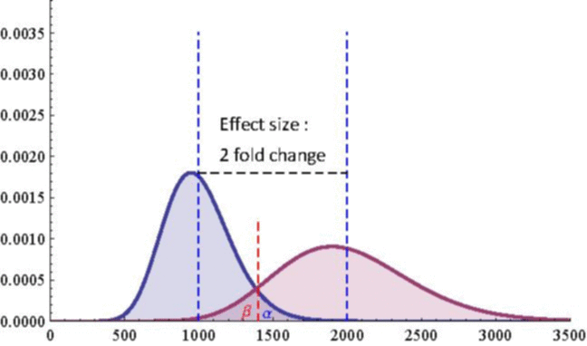
For a single replicate, the sampling distributions in the control and case condition are identical to the negative binomial distributions
and the calculation of \(\beta\) is illustrated on the following figure.
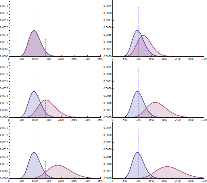
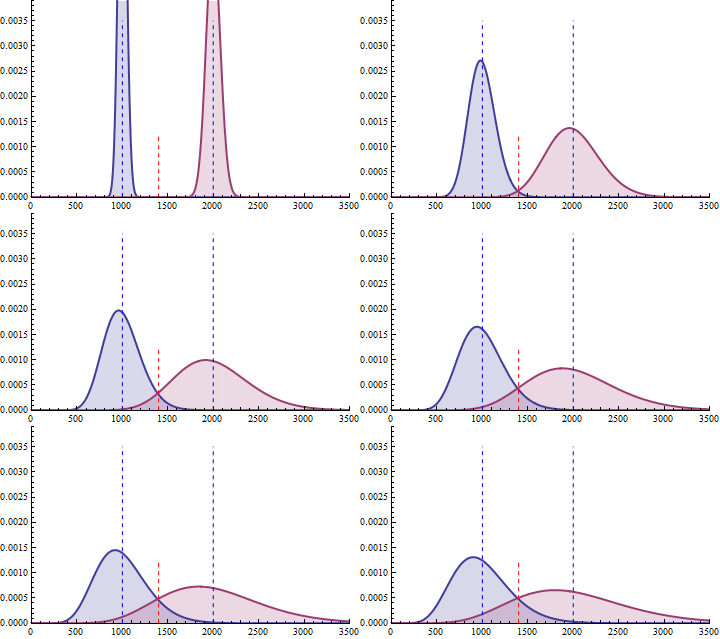
The next 2 figures illustrate the impact of effect size (left animation) on the statistical power to detect a significant fold change on gene expression in RNA-seq data for two
negative binomial distributed read counts and impact of dispersion (right animation) with unchanged effect size but with heterogeneity parameter ranging from 0.001 to 0.10.
On the left animation, the heterogeneity parameter is kept identical for both negative binomial distributions
NB2(\(\mu\), 0.05).
The red dashed line indicates the threshold for a 5% risk of false positive under the assumption that there would
be no differential expression across the sample conditions in the case a NB distributed population with mean 1000
and heterogeneity parameter = 0.05.
For a negative binomial distribution of mean 1000 and heterogeneity
parameter = 0.05, the threshold is 1398 with type I error = 0.05 (for type I error = 0.01 it is 1598) for a
single biological replicate per condition.
For a sample size of 3 (resp. 4), the empirical sampling distributions are simulated
with 50.000 repeats of the sampling procedure and by computing the 99% quantile of the mean under the null assumption
to determine the fold change threshold that will serve to compute \(\beta\) under the assumption of a 2-fold effect size
in the alternative hypothesis. \(\beta\) was computed as the number of times (divided by 50.000 repeats) where the mean of the cases were smaller
than the 99% quantile of the mean under the null.
The empirical sampling distribution under the null and the alternative hypotheses are displayed on the following figures.
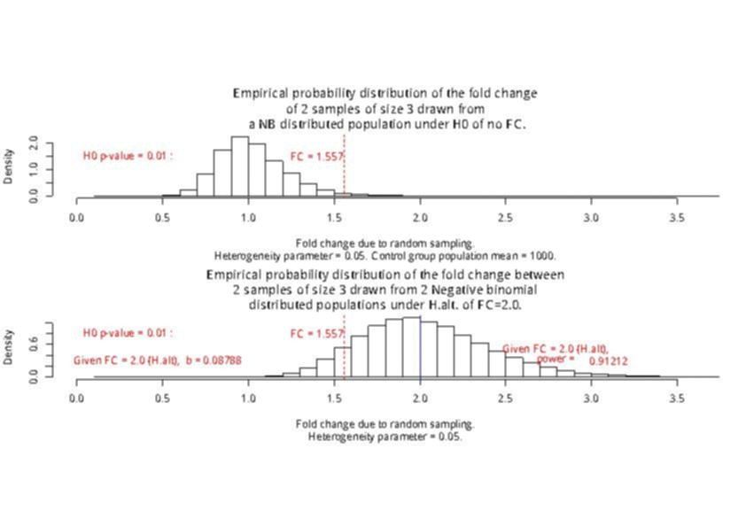
As a conclusion, with a sample size of 3 per condition, we see that the experimental setting is powered enough (power > 0.91) to detect a 2-fold change in gene differential expression across the conditions, while controlling type I error to 0.01 for a single test.
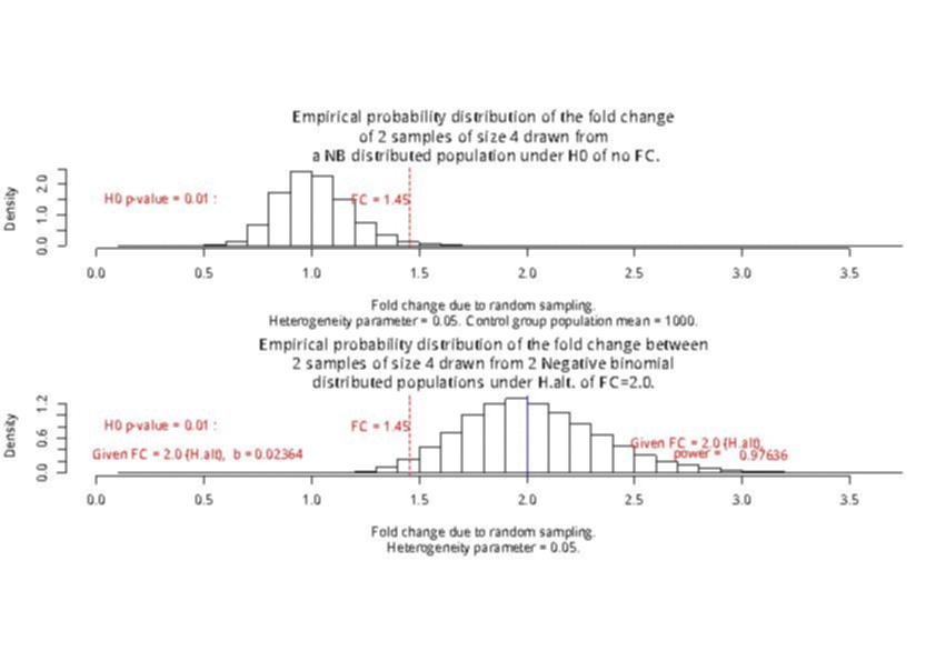
With a sample size of size 4 per condition, the power is higher than 0.97 to detect a 2-fold change in gene differential expression across the conditions, while controlling type I error to 0.01 for a single test.
Multiple testing
Credits: Efron, B. Hastie, T. Computer Age Statistical Inference. Chap. 15: Large Scale Hypothesis Testing and False-Discovery Rates. Cambridge University Press, 2016.
For many statisticians, microarrays and later RNA-seq high-throughput technologies provided an introduction
to large scale data analysis and raised the need to carry out thousands of simultaneous hypothesis testing, done with
the prospect of finding only a few interesting genes among a haystack of null cases.
Testing multiple hypotheses can result in an inflation of the type I error rate (false positive, e.g. rejecting
the null given that the null is actually true).
The most troubling fact about large-scale testing is how easy it is to be fooled.
Recall that, in practice, if \(\alpha=0.05\) is the type I error for a
single case hypothesis test, then, if \(N\) independent tests are conducted, the probability that no error is made
is \((1-\alpha)^N\). Hence, the probability that at least one hypothesis will be rejected wrongly is \(1-(1-\alpha)^N\).
Suppose we conduct 100 tests, then the probability to reject wrongly at least one test out of the 100 is 0.994. It is
almost certain that we will have at least one false positive result. With \(\alpha=0.01\), the previous probability
would still be 0.634.
We see that when the number of tests (supposed here to be mutually independent) is huge, it is almost certain that
we will reject wrongly a great number of tests and will declare a large number of false positives.
How can we adjust for the multiple testing issue ?
Bonferroni multiple testing adjustment
In the Bonferroni multiple testing adjustment, \(\alpha\) is lowered so as to minimize \(1-(1-\alpha)^N\). For instance,
with 100 tests, \(\alpha\) must be set to 0.0005 for the multiple family-wise error rate (FWER) to be less
than 0.05. With thousands of
tests, \(\alpha\) still need to be much more minimized and this is detrimental to the statistical power.
The Bonferroni correction for multiple testing (where the single case test \(\alpha\) is divided by the number of tests \(N\))
is not fully exact because the independence of tests does not hold for gene
expression and the Bonferroni adjustment is too conservative. The Bonferroni adjustment is better suited for a number
of tests \(N\) between 2 and perhaps 20.
False-Discovery Rates
The family wise error criterion (FWER) aims to control the probability of making even one false rejection among \(N\)
simultaneous hypothesis tests. Originally developped for small-scale testing, say \(N \le 20\), FWER usually proved too
conservative when working with \(N \sim \) thousands.
A quite different and more liberal criterion, the false discovery rate (FDR) has become standard.
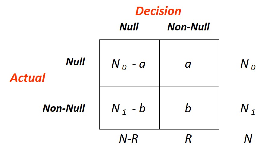
The figure here on the right, taken from Efron and Hastie (2016), diagrams the outcome of a hypothetical decision rule \(D\)
applied to the data for \(N\) simultaneous hypothesis-testing problems, \(N_0\) null and \(N_1=N-N_0\) non null. An
omniscient oracle has reported the rule's results: \(R\) null hypothesis have been rejected: \(a\) of these were cases of
false discovery, i.e., rejected valid null hypothesis, for a false-discovery proportion (Fdp)
\begin{equation}
Fdp(D) = \frac{a}{R}
\end{equation}
\(Fdp\) is unobservable: without the oracle we cannot see \(a\), but under certain assumptions we can control its expectation.
Define
\begin{equation}
FDR(D) = E[Fdp(D)]
\end{equation}
A decision rule \(D\) controls FDR at level \(q\), with \(q\) a prechosen value between 0 and 1, if
\begin{equation}
FDR(D) \le q
\end{equation}
It might seem difficult to find such a rule, but in fact a quite simple but ingenious recipe does the job.
Ordering the observed p-values from smallest to largest:
\begin{equation}
p_{(1)} \le p_{(2)} \le p_{(3)} \le \cdots \le p_{(i)} \le \cdots \le p_{(N)}
\end{equation}
Define \(i_{max}\) to be the largest index for which
\begin{equation}
p_{(i)} \le \frac{i}{N}\,q
\end{equation}
and let \(D_q\) be the rule that rejects \(H_{0(i)}\) for \(i\le i_{max}\), accepting otherwise.
The Benjamini-Hochberg FDR Control theorem states that:
If the p-values corresponding to valid null hypotheses are independent of each other, then
\begin{equation}
FDR(D_q) = \pi_0 q \le q
\end{equation}
where \(\pi_0=\frac{N_0}{N}\)
- Classic theory is purely frequentist, whereas false-discovery rates combine frequentist and Bayesian thinking.
- In classic testing, the attained significance level for case \(i\) depends only on its own test statistic score \(z_i\), while \(\hat{fdr}(z_i)\) or \(\hat{Fdr}(z_i)\) also depends on the observed test statistics for other cases.
- Applications of single-test theory usually hope for rejection of the null hypothesis with familiar prescription being 0.80 power and type I error set to 0.05. The opposite is true for large-scale testing, where the usual goal is to accept most of the null hypothesis, leaving just a few interesting cases for further study.
- False-discovery rate hypothesis testing involves a substantial amount of estimation, blurring the line between frequentism and Bayesianism, the two main branches of statistical inference.
Differentially expressed gene sets interpretation: gene ontology, gene set enrichment analysis, enrichment maps, networks, pathways
Credits: Daniele Merico, Ruth Isserlin, Oliver Stueker, Andrew Emili, Gary D. Bader. Enrichment Map: A Network-Based Method for Gene-Set Enrichment Visualization and Interpretation. PloS ONE5(11), 2010.Christophe Dessimoz, Nive Skunca. The Gene Ontology Handbook. SpringerOpen, 2017.
The output of high throughput genomic experiments is typically a large gene list ranked by their differential
expression between two biological states (across two conditions, between two cell types, across time points series,
etc...).
However, these large gene ID ranked lists are not easy to interpret and the formulation of consistent biological
hypotheses from these results still poses a major challenge for experimental biologists.
At first, the biological explicite description or the gene product properties associated to a gene tag ID
must be determined by searching annotated databases and the so called Gene Ontology databases.
The purpose of gene ontology (controlled formal vocabulary of gene and gene products) is to map the gene IDs to curated and
annotated terms relevant to the biological properties of all the gene tags of interest: cellular components,
molecular functions and involved biological processes. A direct mapping of the gene tag IDs to annotated gene description can be done, for instance,
in Cytoscape with GeneMania app or using GSEA (Gene Set Enrichment Analysis) web resources.
Enrichment analysis is an automated and statistically rigorous technique to analyse and interpret large gene lists
using a priori-knowledge. Enrichment analysis assesses the over- (or under-) representation
of a known set
of genes (e.g. a biological pathway) within the input gene list. If a statistically significant larger number of
genes from the known set are present in the gene list, it may indicate that the biological pathway plays a role
in the biological condition under study. This analysis is repeated for all available known gene-sets, which
could number in the thousands.
There are plenty of enrichment analysis methods and tools. They mainly differ in their database of known
gene-sets and the statistical method used to asses enrichment.
Gene sets can be defined based on participation in a metabolic or signaling pathway (e.g. KEGG, REACTOME,
targeting by gene expression regulators like microRNA or transcription factors), etc.
Statistical methods to determine enrichment are usually either threshold-dependent (Fisher's Exact Test)
or whole-distribution (GSEA). Threshold-dependent techniques require the user to input a discrete list of
top-ranking genes, which may require setting a threshold on the gene scoring statistic. The one-tail Fisher's
Exact Test, based on the hypergeometric distribution, is the golden standard method used. A shortcoming
of this method, however, lies in the loss of information caused by treating gene scores in a binary way
(they either pass the threshold or not).
On the other hand, whole distribution methods are threshold-free, as they test gene-sets by comparing
their score distribution versus the background distribution.
The Fisher test for enrichment analysis:
the gene-category analysis cast the problem as a statistical test. The actual outcome of the study is referred to as
the study set (= the differentially expressed genes in the daaset). The population set is the set
of all the mapped genes in the RNA-Seq experiment (all the genes of the dataset). The study set is assumed to be a
random sample that is obtained by drawing $n$ items without replacement from the population. The population is
dichotomic as the items can be characterized according to whether they are annotated to term \(t\) or not.
In particular, the set \(M_t\) with cardinality \(\# = m_t\) constitutes all items that are annotated to \(t\). Denote the
random variable that describes the number of items of the study set that are annotated to \(t\) in this random sample
as \(X_t\). The hypergeometric distribution applies to \(X_t\) and the probability of observing exactly \(k\) items annotated to \(t\), i.e., \(P(X_t\,=\,k)\) is specified by
\begin{equation}
P(X_t=k) = \frac{
\begin{pmatrix}
m_t\\k
\end{pmatrix}
\cdot
\begin{pmatrix}
m-m_t\\
n-k
\end{pmatrix}
}{
\begin{pmatrix}m\\
n
\end{pmatrix}}
\end{equation}
In the study set (\(N\)), you have cardinality \(n\) with \(n_t\) annotated to the term \(t\). The objective
is to assess whether the study set is enriched for term \(t\), i.e., whether the observed \(n_t\) is higher
than one would expect by chance alone. This forms the alternative hypothesis \(H_1\) of the statistical test. The
null hypothesis \(H_0\) in this case is that there is no positive association between the observed occurence of
the itmes in the study set and the annotation of the items to the term \(t\). Thus, the proportion of items
annotated to term \(t\) is approximatively identical for the study set and the population set. In order to reject
\(H_0\), we conduct a one-sided test in which we compute the probability to see \(n_t\) or even a larger number of
annotated items given that \(H_0\) is true. If the probability obtained is below a chosen fixed significance level
\(\alpha\), e.g. \(\alpha \le 0.05\), we reject \(H_0\).
Example of a Fisher test for enrichment analysis:
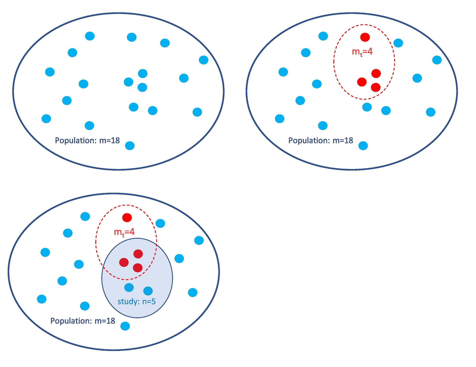 Suppose that we are given a population of \(m=18\) genes, of which \(m_t=4\) genes are annotated to term \(t\) (red).
The outcome of the experiment yields a study set of \(n=5\) differentially expressed genes. A total of \(n_t=3\)
genes from the genes of the study set are annotated to \(t\) (are red).
What is the probability to have in the study set 3 (or more) genes annotated to term \(t\) if they had been randomly sampled ?
\begin{equation*}
P(X_t \geq 3 \mid H_0) = \frac{
\begin{pmatrix}
4\\
3
\end{pmatrix}
\cdot
\begin{pmatrix}
18-4\\
5-3
\end{pmatrix}
}{
\begin{pmatrix}18\\
5
\end{pmatrix}}
+
\frac{
\begin{pmatrix}
4\\
4
\end{pmatrix}
\cdot
\begin{pmatrix}
18-4\\
5-4
\end{pmatrix}
}{
\begin{pmatrix}18\\
5
\end{pmatrix}}
= 0.044
\end{equation*}
The p-value is \(0.044 (<0.05)\) and it is considered too rare to have occurred just by chance.
So \(H_0\) is rejected and the study set is indeed enriched in genes annotated to term \(t\).
The study set is indeed enriched in the red genes, as can be seen from the large overlap between
the study set and the subset of the red genes in the population set.
Enrichment Map: to simplify the navigation and interpretation of enrichment results,
a network-based gene-set enrichment result visualization method has been developped by
Bader lab, 2010 (see credits above). What is an enrichment map ?
Gene-sets are first analyzed for
enrichment significance using a method of choice (GSEA for instance), and then organized as weighted
similarity network (undirected weighted graph), where nodes represent gene sets (gene ID elements belonging to
a given pathway for instance) and weighted edges between the nodes represent
an overlap score depending on the shared number of genes between two gene-sets. The size of a node
is made proportional to the number of genes it contains (cardinality, \(\#\), of the gene-set). The overlap score writes:
\begin{equation}
\text{overlap} =\frac{\#(A\cap B)}{min\{\#A,\, \#B\}}
\end{equation}
The thickness of the edges is made proportional to the overlap score between the two connected nodes.
We illustrate hereafter a comparison of two enrichment maps describing the most significant REACTOME pathways
that were enriched on RNA-Seq data experiments contrasting LEC (Lymphatic endothelial cells) grown a tumor
secretome medium; or LEC grown under VEGF-C (Vascularisation Endothelial Growth Factor-C) as compared to a
control medium in both cases.
The LEC cells grown on a tumoral medium (left panel below) show enrichment in pathways related to cell-cell signalling
activities: chemokines-cytokines secretion while lipids metabolism and cholesterol biosynthesis are
down-regulated.
The LEC cells grown on VEGF-C (right panel below) show enrichment in pathways related to cell mitotic activities, proliferation
and cell migration.
